
For developing the tensile roof two similar yet different approaches were taken up. In the first approach a MESH PLANE component was taken up, where as in the second one a MESH BREP.
Result of Approach 1:

OPTION 1- Mesh Plane
Result of Approach 2:
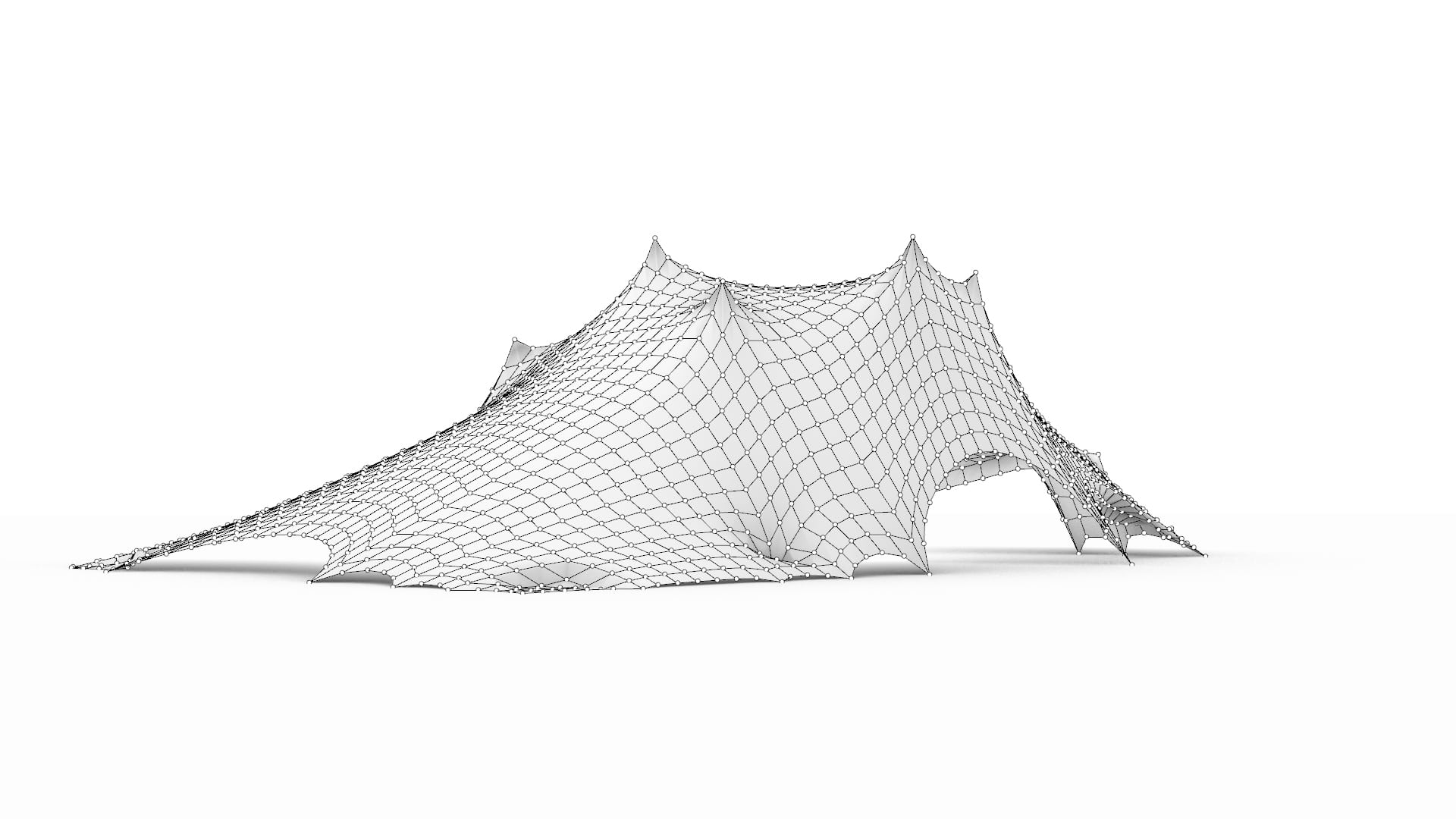
OPTION 2- Mesh Brep
The tensile roofing is designed to replace the bamboo roof structure of the complex with a more Dynamic tensile form.
Initial Concept of the Museum Complex:
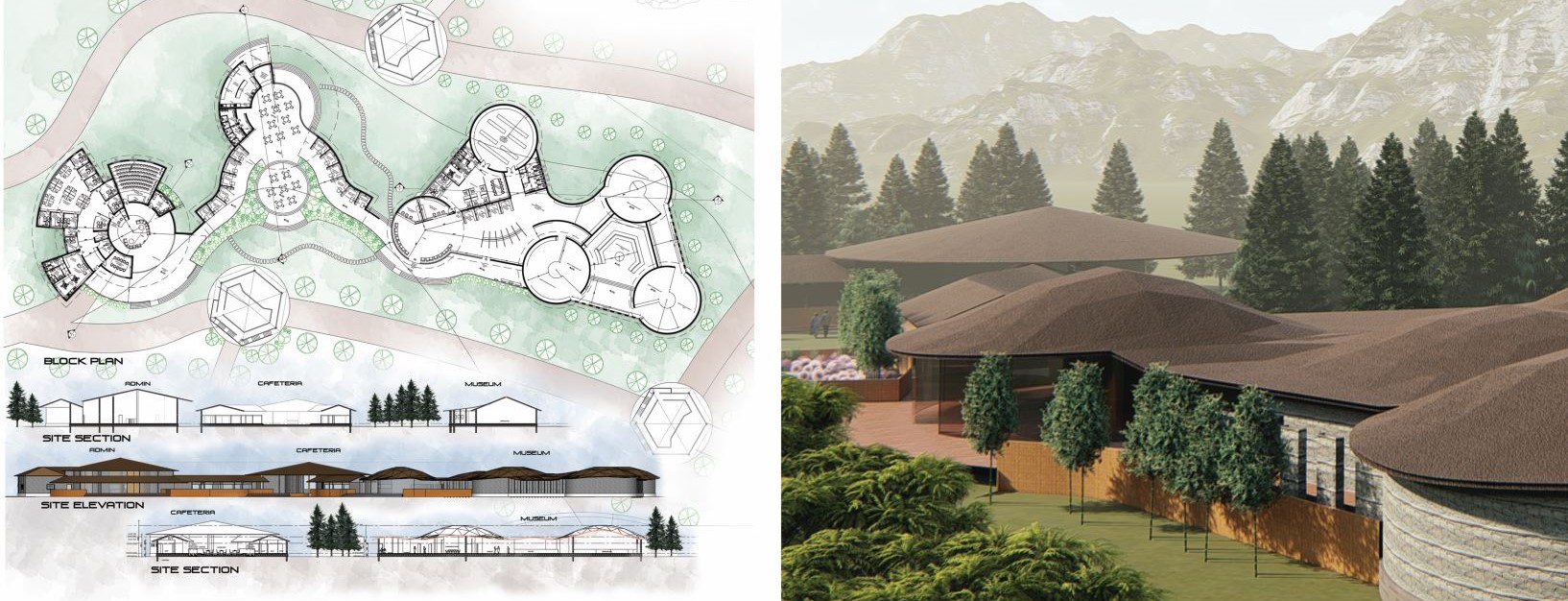
Initial Design of the Museum
The view of the globular bamboo roofing.
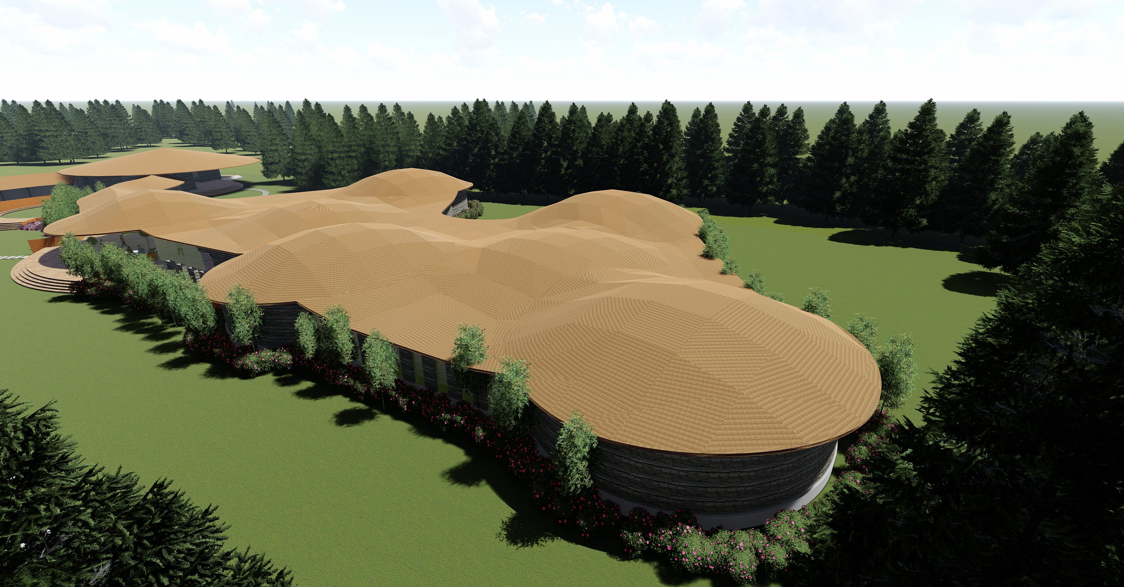
The Globular Roof form.
Replacing the Globular roof structure of the Museum with a more Dynamic form using Kangaroo and Weaverbird.
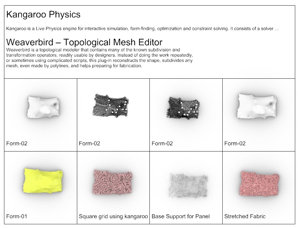
Kangaroo Physics
Kangaroo is a live Physics Engine for interactive simulation, form-finding, optimization and constraint solving.
It works with the inputs such as:
– Show
– Anchor Points
– Load Points
– Edge Length
– Solver
Weaverbird- Topological Mesh Editor
Weaverbird is a topological modeler that contains many of the known subdivisions and transformation operators, readily usable by designers. Instead of doing the work repeatedly, or sometimes using complicated scripts, this plug-in reconstructs the shape, subdivides any mesh, even made by polylines, and helps in developing fabrication for the structure.
Concept- The evolution of Project
STEP 1: Setting of a curve.
Setting of a curve and creating a mesh plane.
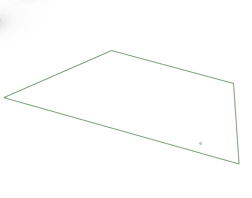
Setting of a curve in Rhino using the component “CURVE”.
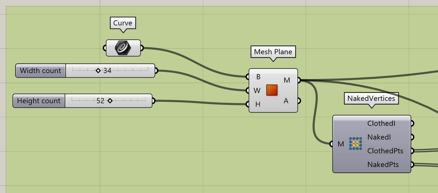
Setting of a Mesh Plane using the component “MESH PLANE”.
Mesh Plane has 3 inputs Boundary(B), Width count(W) and Height Count(H). Where boundary is the curve we set in step 1, Width count is the number of faces along X direction and Height count is number of faces along Y direction. Both width count and Height count are set using Number sliders which can control the size of the mesh. The output of the component is a Mesh(M) and its area.
When we use the component MESH PLANE always develop a rectangular plane as the input data is the width and the height count.
Setting of Vertices on the Mesh Plane with the component “NAKED VERTICES”.
Naked vertices component has a Mesh as an input and the outputs are Clothed Index, Naked Index, Naked Points and Clothed Points. Naked points are the points along the periphery of the mesh and the clothed points are the points inside the periphery. Clothed index output and Naked index output gives the indexes of vertices surrounded by faces.
Selection of Naked Points.
Selection of Clothed Points.
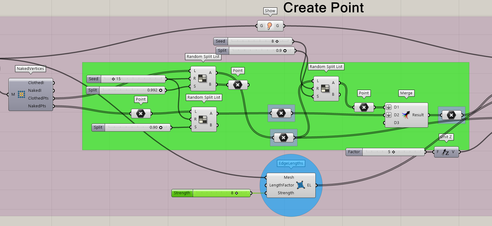
Step 2: Generating of Anchor Points and Load Points.
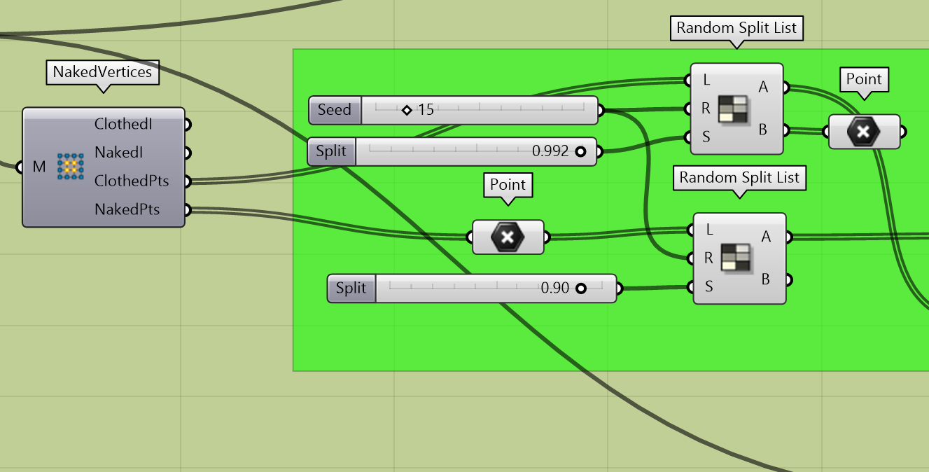
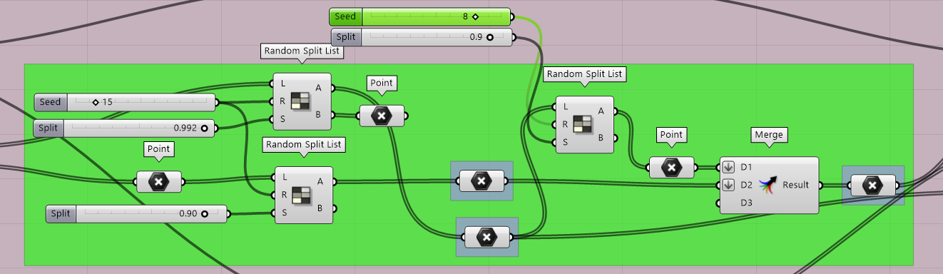
Using Random split component to create a list of points that will act as Load points and Anchor Points
Random Split List it splits a list into 2 lists. The inputs of the component are Master list (L), Seed(R), and Split(S); the outputs are two lists A and B. We load the clothed points to a Random split list into the Master List input and the naked points into another to derive the Random points that will acts as Load Points and Anchor points of the Structure (Skin). The split value is inserted using a number slider, which can define the ratio in which the list will be split; for instance 0.5 will give us 50:50 list, where as 0.25 will give a 25:75 etc. The seed value helps us in deriving with probable set of points.
Random selection of points using Random Split List

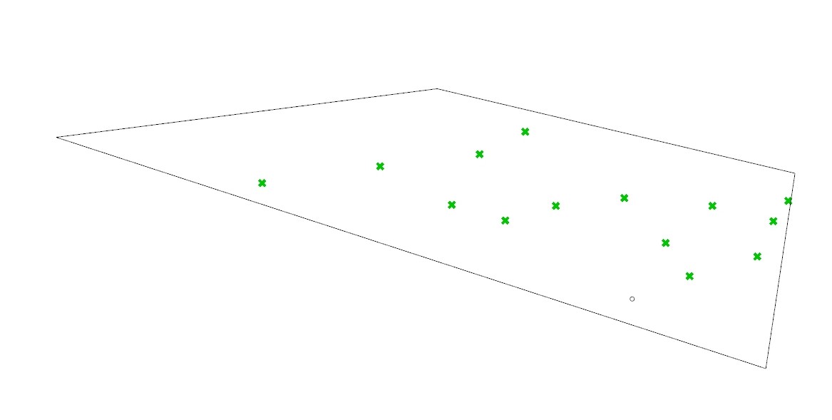
The output preview of the Randomly selected Anchor Points generated from Naked Points using Random Split List.

The output preview of the Randomly selected Load Points generated from Clothed Points using Random Split List.
Selection of High points of the structure.
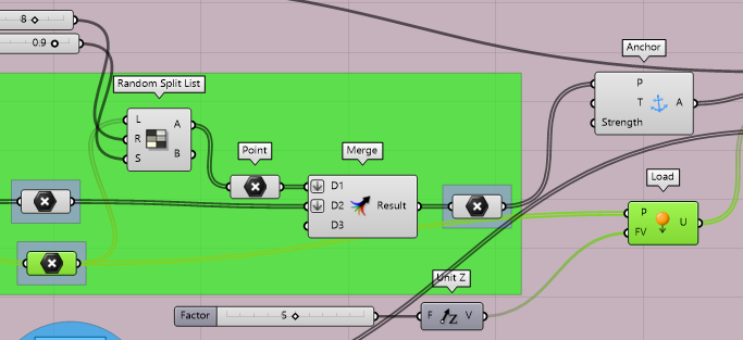
Step 3: Derivation of final set of points.
Derivation of Final Set of Load Points, Anchor Points and High Points.
The Output preview of the final set of Load points, Anchor Points and High Points.
The set of the final set of Anchor points, Load points and the high points are fed to MERGE component and stored inside the POINT component.
Step 4: Anchor Component and Load Component
The Load points derived from clothed points are fed into the component “LOAD”.
The load points that are fed to LOAD
The set of Anchor points derived from Naked points are fed into the component Anchor.
From the Random Split component we get the output of a set of points (as lists), which will be the final set of Anchor points, Load Points and High Points of the structure. The set of Load point list are further added to the component LOAD. The component LOAD has two inputs- Point(P) and Force Vector(FV). A Unit Z factor in a positive Z value is connected to force vector where we input the load that will be applied to the structure and will define the form. Unit Z factor will act along the Z direction and it will specify the highest point of the roof structure. The positive Z value is added as we want to set the highest point of the structure.
The Anchor Command has the inputs Point(P), Target(T) and Strength, where we feed the points into the command and the output is the Anchor out. It sets the final anchor points of the structure before fed into the BASIC SOLVER.
Step 5: Show and Edge Lengths
 Edge length is a command is used to determine the strength or the force that the structure can withstand.
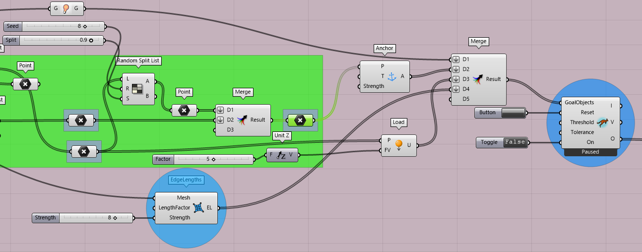
The values derived from Anchor component, Load Component, Show and Edge length components are first merged using a MERGER and the fed into the Basic Solver. These set of values are the raw input for the Solver.
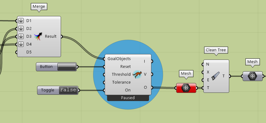
Step 6: Solver
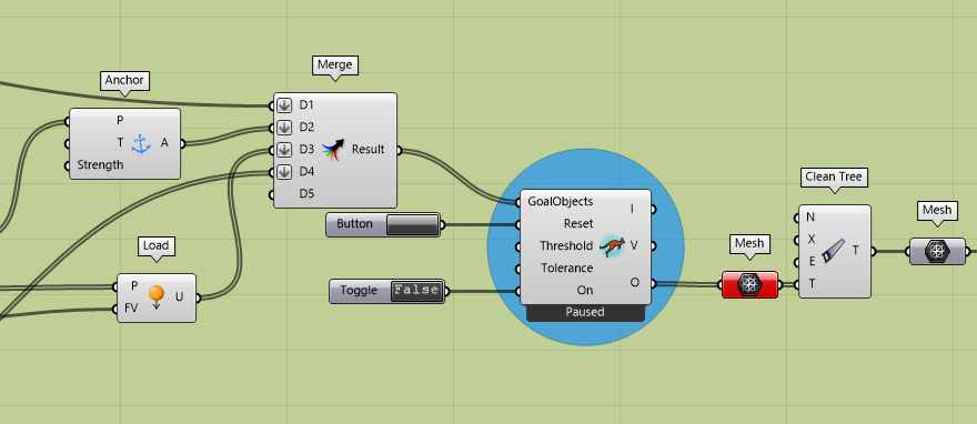
Merging the final set of data to feed into the SOLVER
Once merged we get an output/ RESULT, which will be the Goal Objects input of the basic solver.
SOLVERS in Kangaroo:
There are 5 types of Solvers in Kangaroo, they are:
- BOUNCY SOLVER
- SOLVER
- SOFT & HARD SOLVER
- STEP SOLVER
- ZOMBIE SOLVER
Here we are using a basic SOLVER. The inputs of a SOLVER Component are Goal Objects, Reset, Threshold, Tolerance and On. The Goal Objects here are the data we derived in the previous steps, ie., the Anchor, Load, Edge length and Mesh. The Reset input is a toggle button to completely rebuild the particle list and indexing. The On input is a true or false toggle button. These Toggle buttons enables us to re process the input data and re-process. The output of the Solver is a Mesh. Due to multiple running of the program the output mesh is likely to have NULL POINTS and we use the CLEAN TREE component to delete these null points and get a clean mesh.
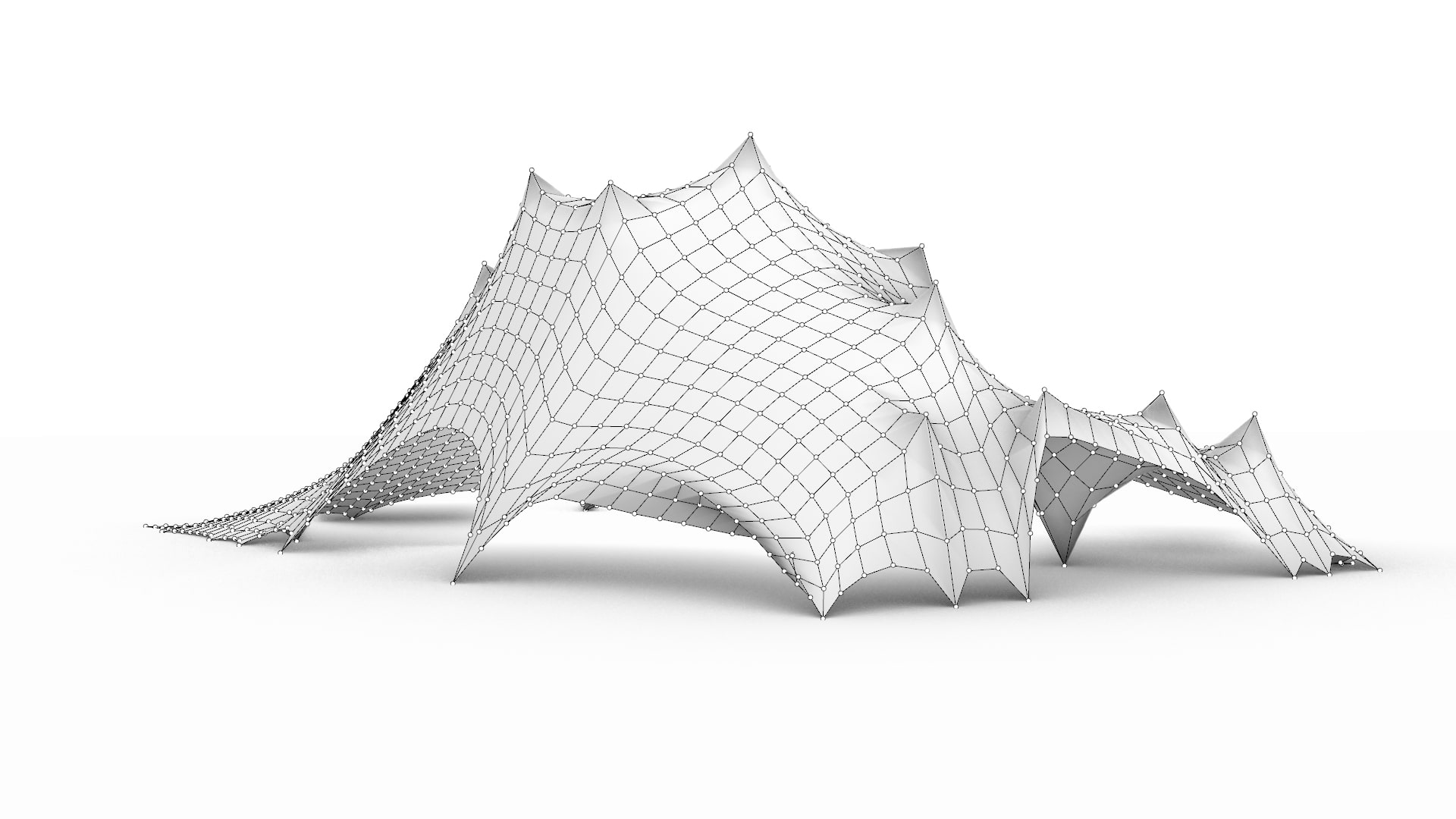
The Mesh Form
Step 7: Visualising
From solver to Mesh
The mesh derived is Deconstructed here to analyse the high points and low points of the structure. Here the lowest point will be depicted in blue and the highest in orange. Once the analysis is done and deriving at the desired mesh form/output we use the Weaverbird plug-in.
Deconstructing mesh- Weaver bird
Weaverbird brings mesh editing, subdivision and mesh transformations.
Realization
The Contour Analysis using Gradient component.
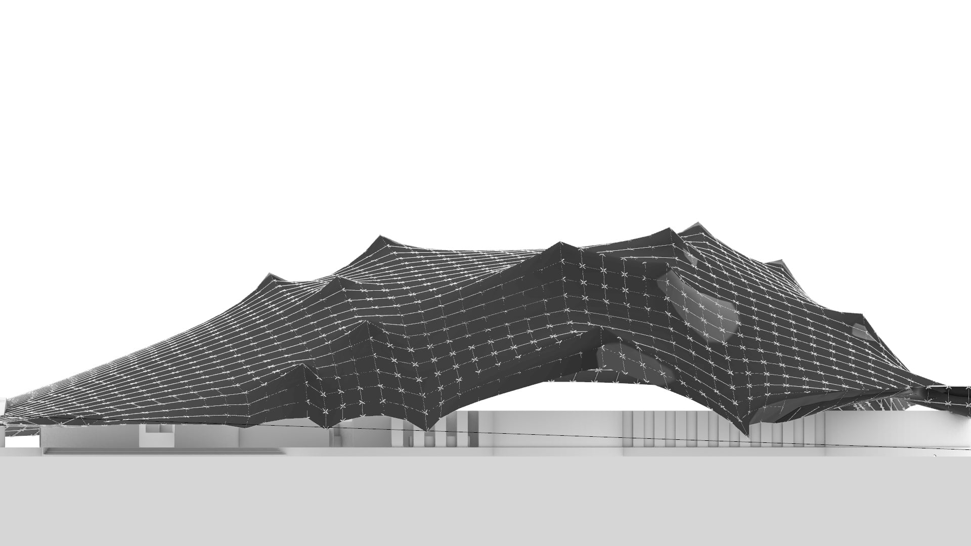
The final script:
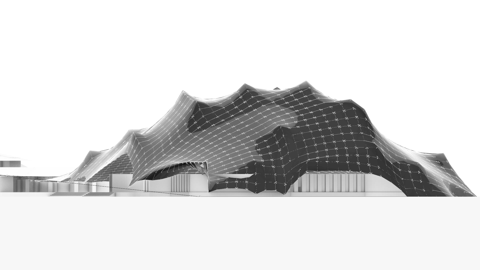
Internal view of the Tensile roofing

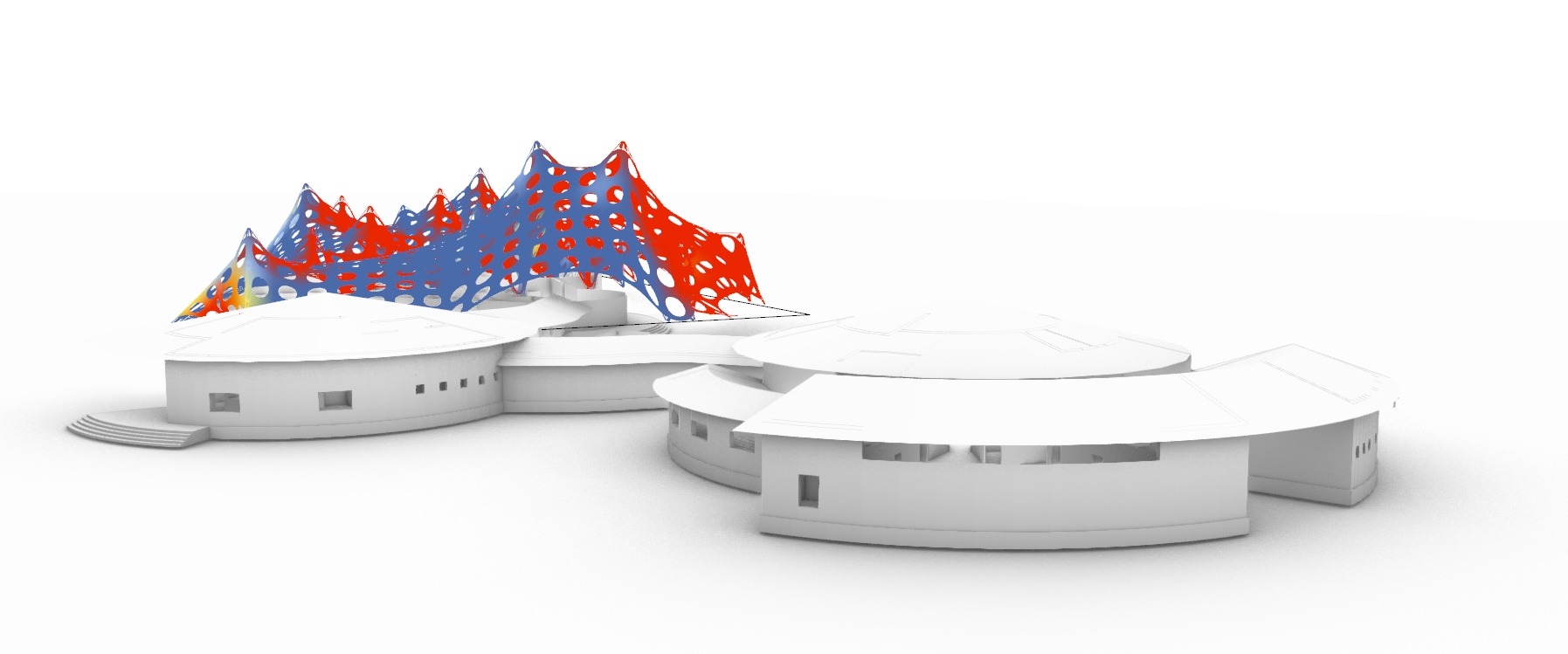
The Tensile Structure
Museum with the updated roofing


FINAL SCRIPT
Grasshopper file- kangaroo 01
Rhino file- 01
APPROACH 2:
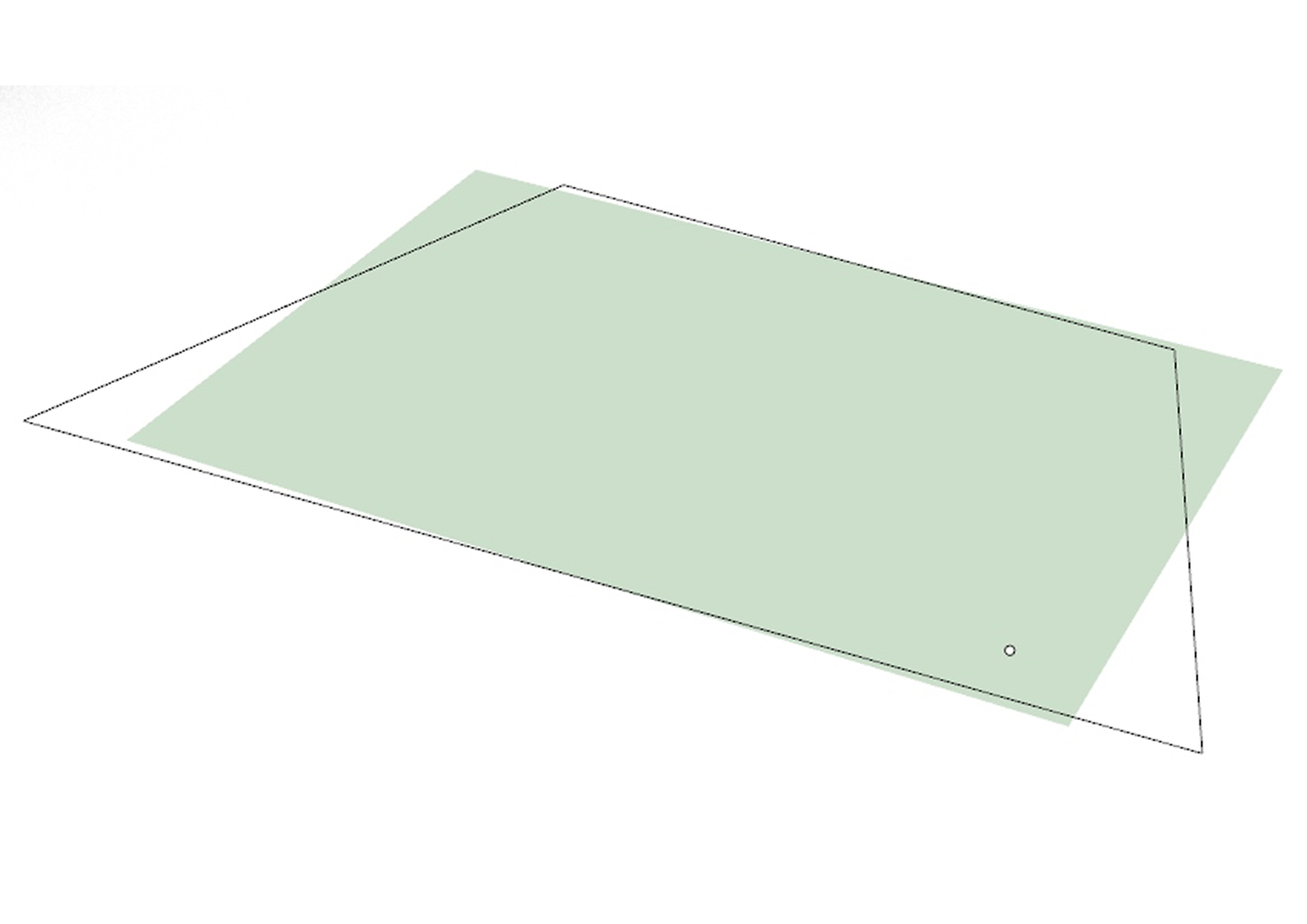
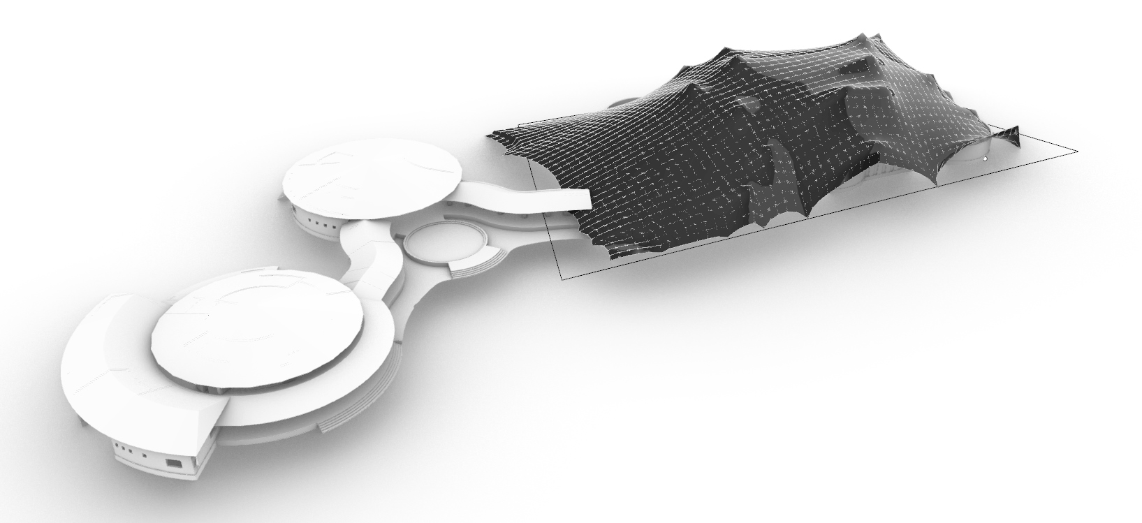
When the MESH PLANE component gets replaced with a MESH BREP component, we get to match the Initial curve with the mesh plane. Here the organic plan of the museum is derived from a trapezium.
STEP 1: Setting of a curve.
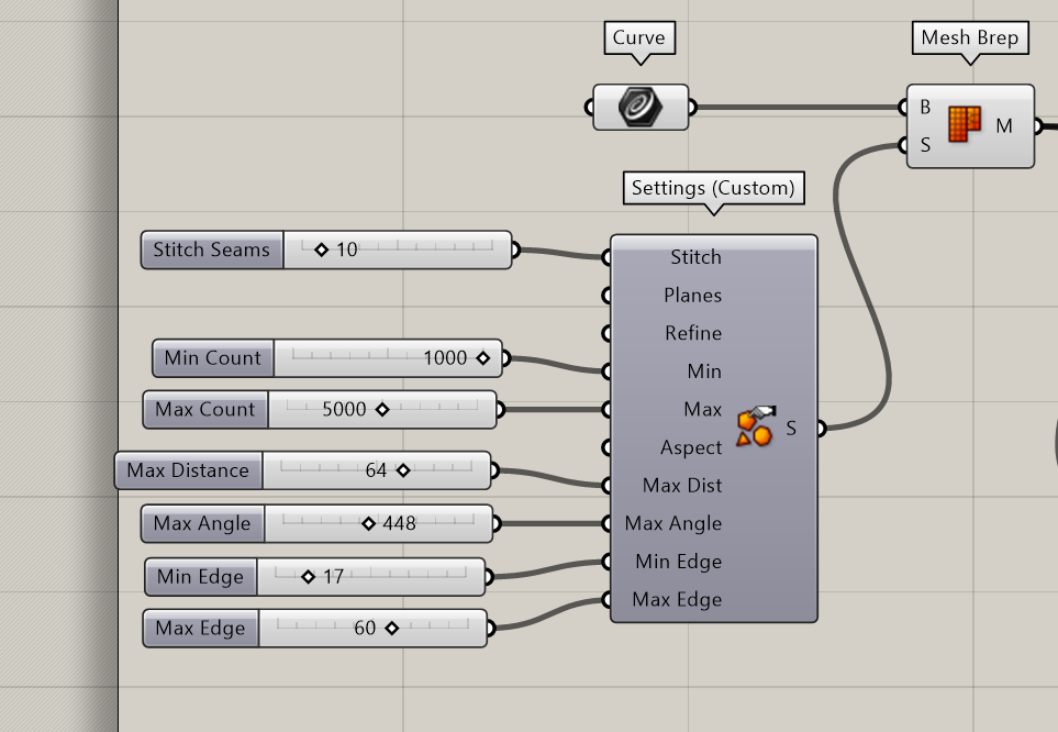
MESH BREP
Mesh BREP-
It has two inputs, brep geometry(B) and settings(S) to be used for the meshing algorithm. Brep is a combination of multiple surfaces.

The Curve
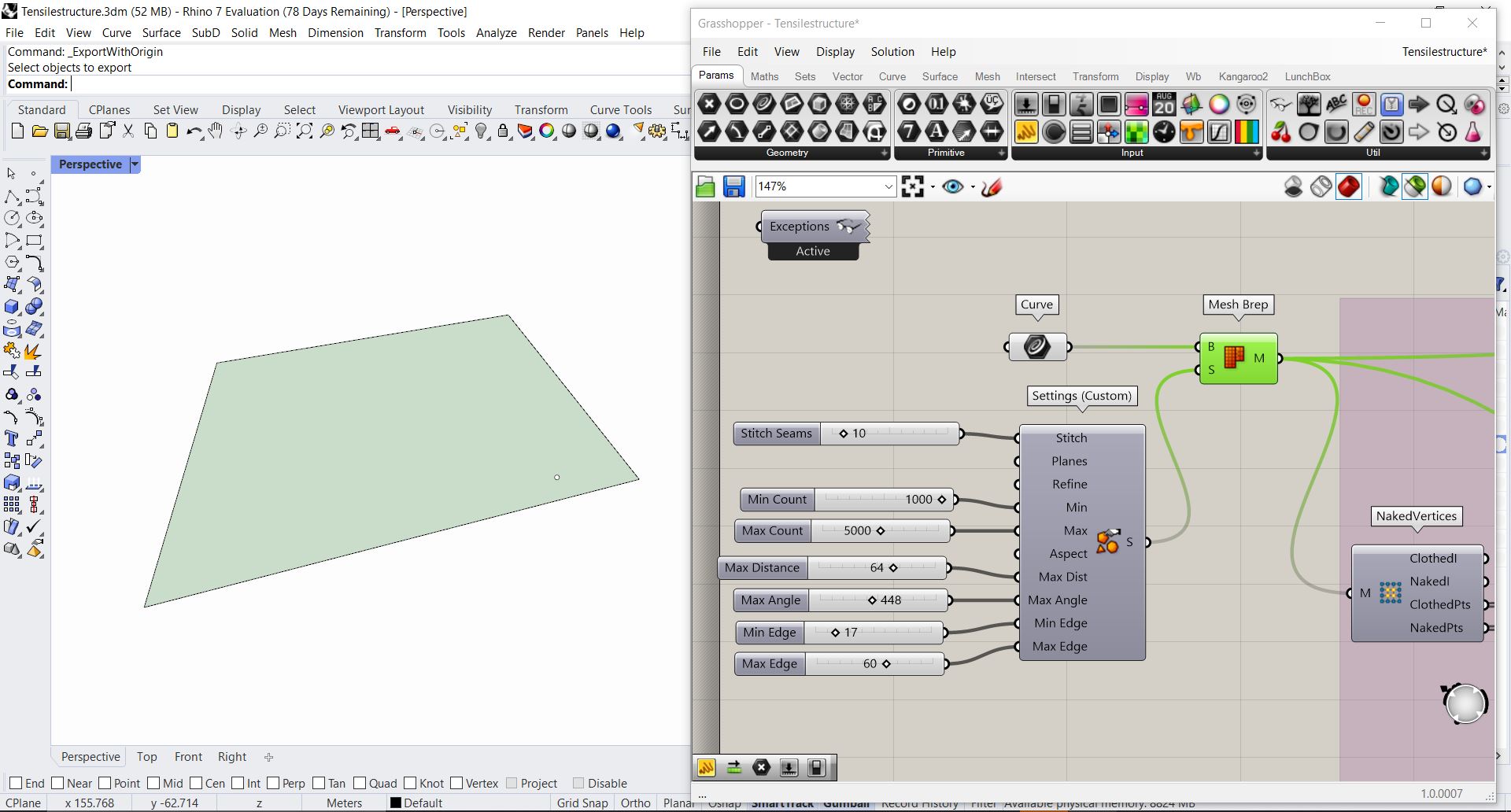
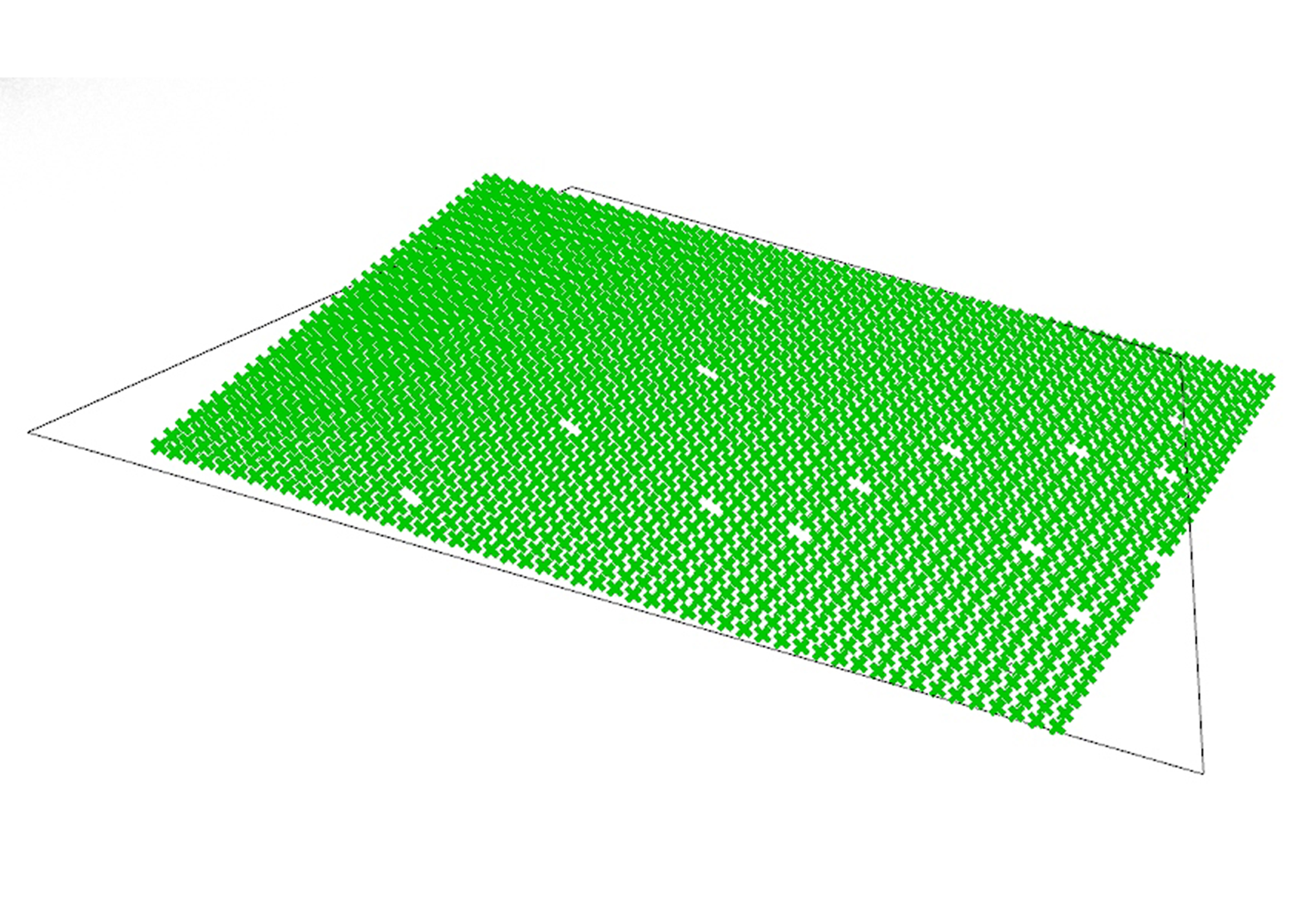
Mesh plane defined using MESH BREP
Step 2: Generating of Anchor Points and Load Points.
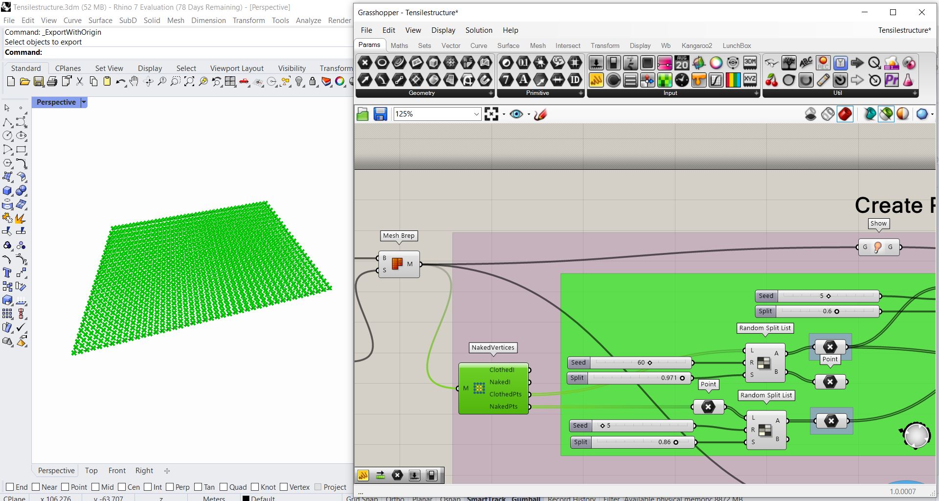
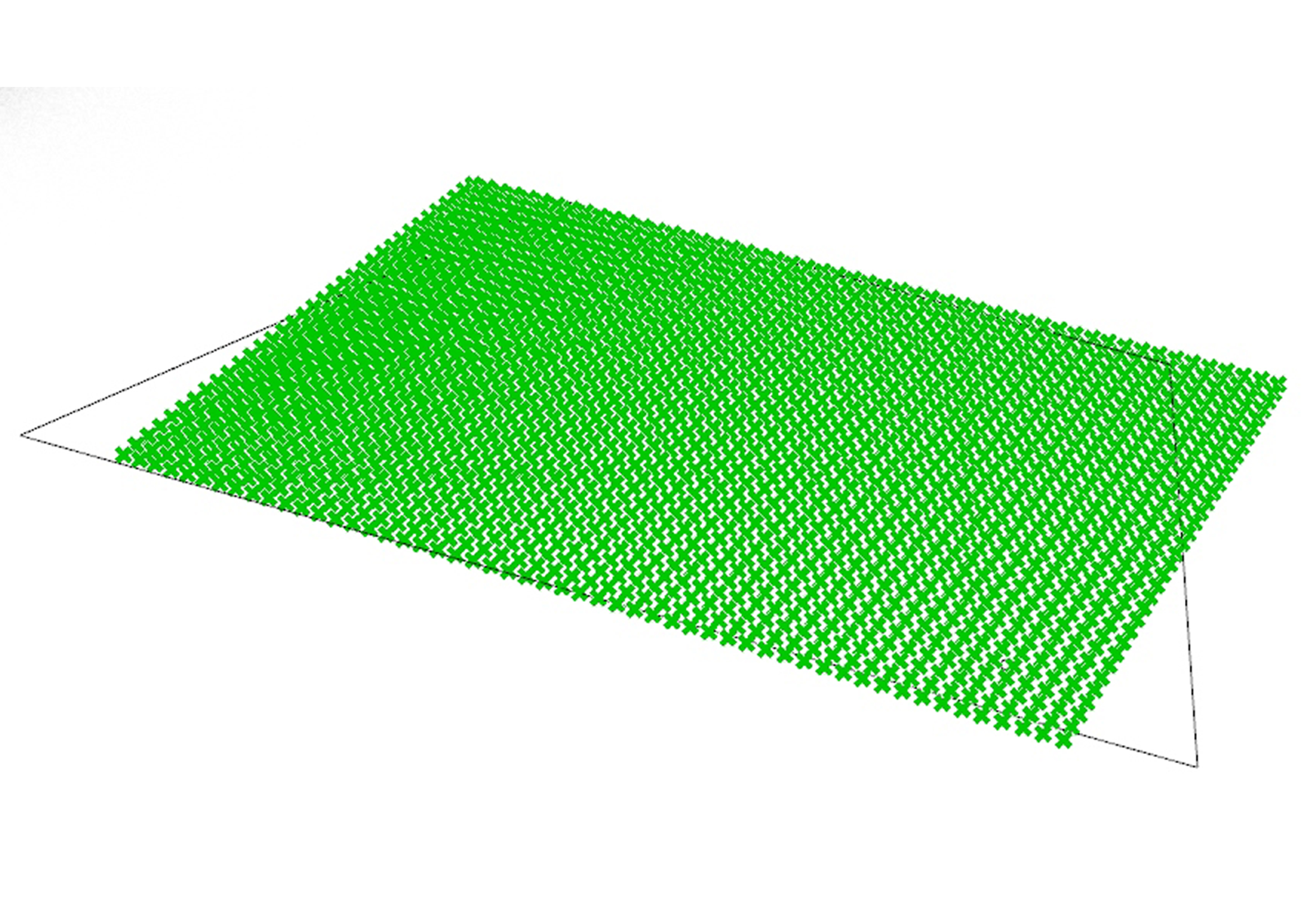
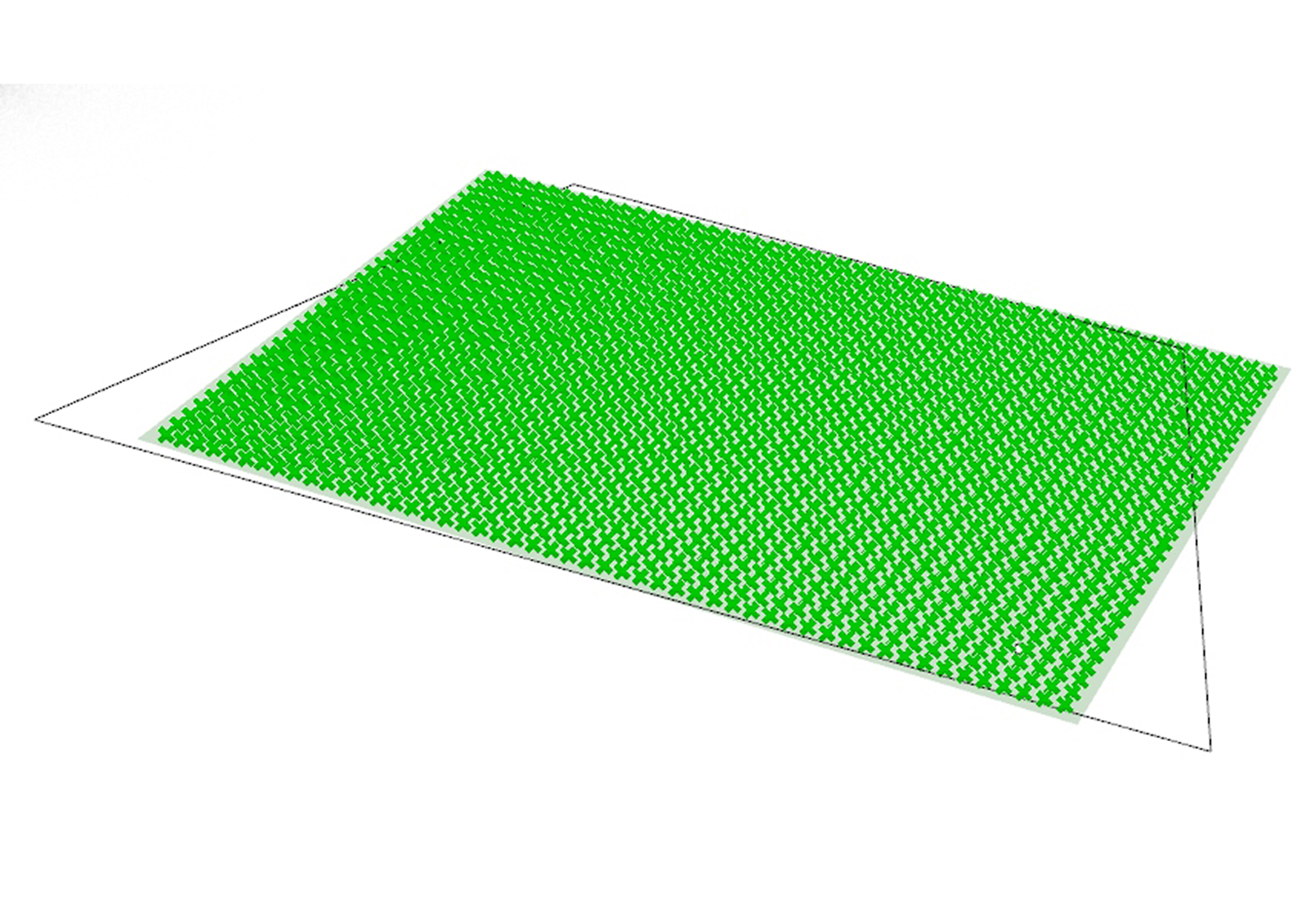
The vertices generated from the mesh plane.
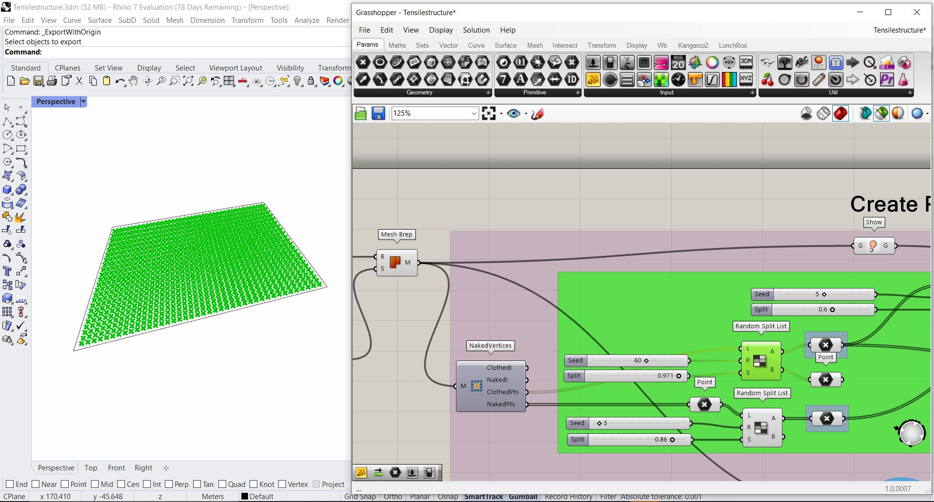
Clothed Points of the Mesh plane.
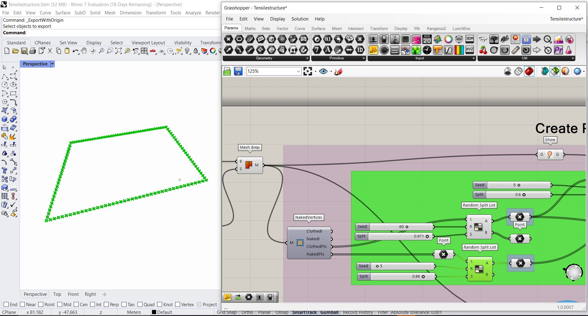
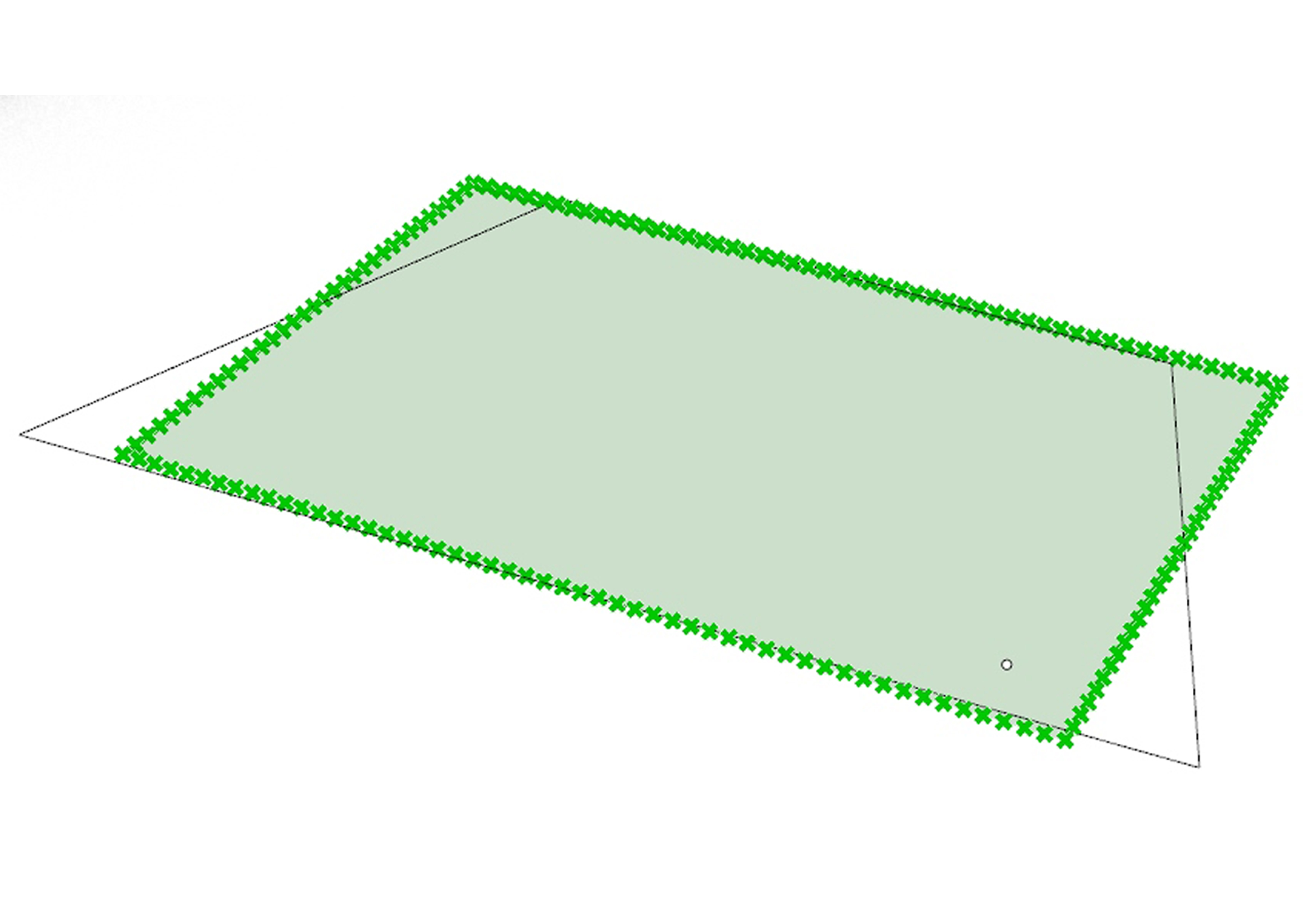
Naked Points of the Mesh plane.

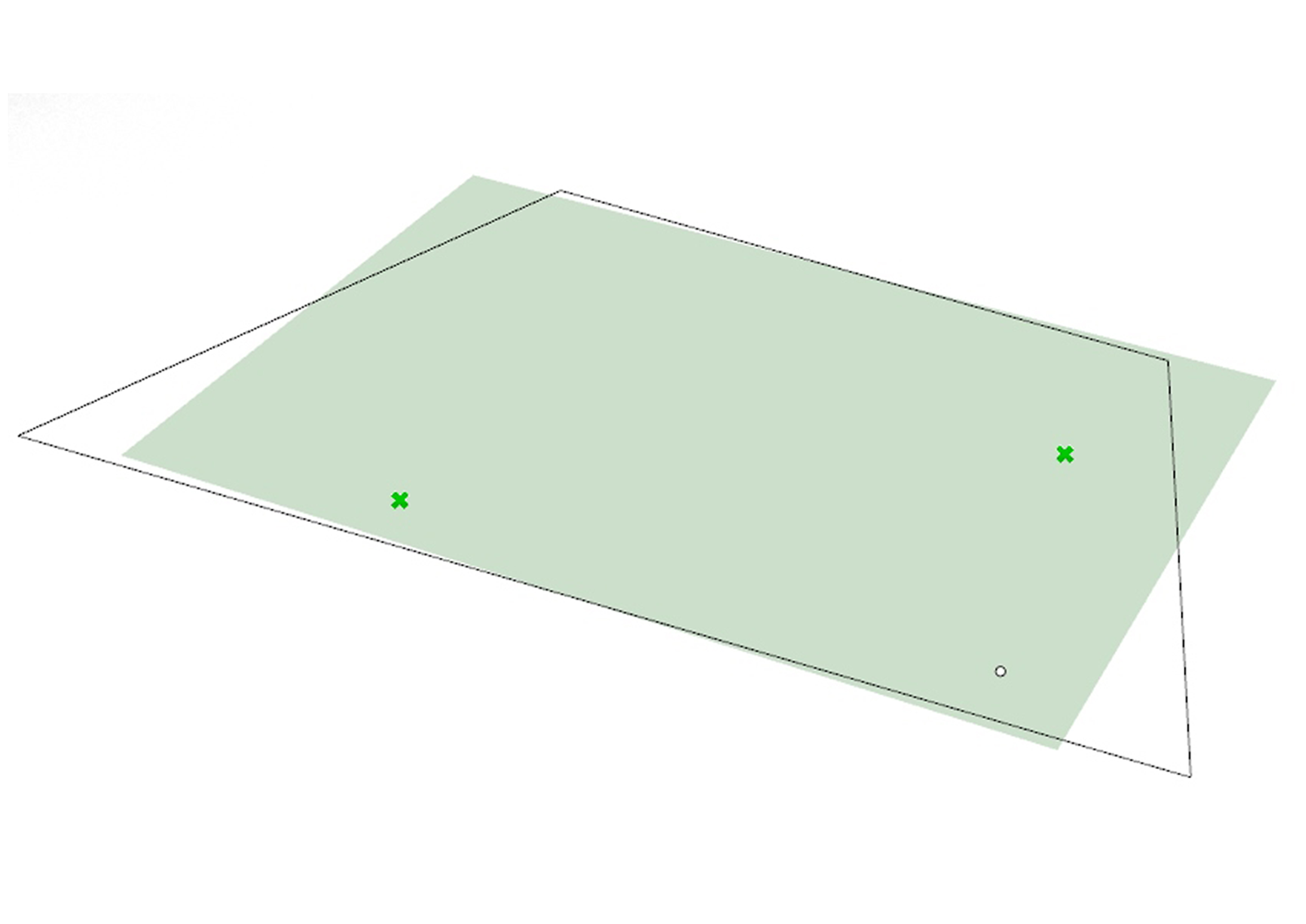
Using Random split to split the set of Clothed points and to choose few points as the load points of the structure.
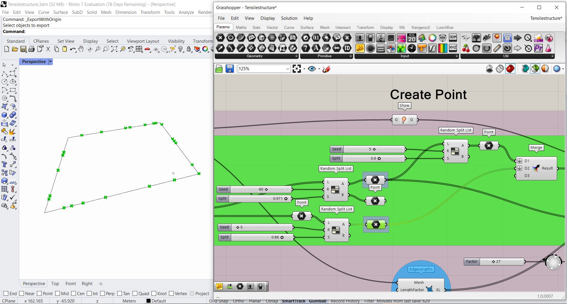
Using Random Split list to generate the set of Anchor points from Naked point list.

Using Random split list to generate the high points from the set of Load points generated.
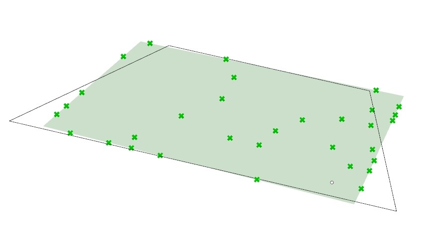
Step 3: Derivation of final set of points.
The final set of Anchor points, load points and high points of the structure merged to derive at the final set of points for the roof structure.
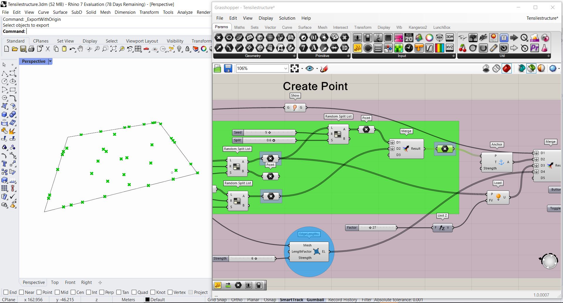
Step 4: Anchor Component and Load Component

LOAD- ANCHOR- MERGE- SOLVER
The Load points derived from clothed points are fed into the component “LOAD” and the set of Anchor points derived from Naked points are fed into the component Anchor.
The component LOAD has two inputs- Point(P) and Force Vector(FV). A Unit Z factor in a positive Z value is connected to force vector where we input the load that will be applied to the structure and will define the form. Unit Z factor will act along the Z direction and it will specify the highest point of the roof structure. The positive Z value is added as we want to set the highest point of the structure.
The Anchor Command has the inputs Point(P), Target(T) and Strength, where we feed the points into the command and the output is the Anchor out. It sets the final anchor points of the structure before fed into the BASIC SOLVER.
Step 5: Show and Edge Lengths
Edge length is a command is used to determine the strength or the force that the structure can withstand.
The values derived from Anchor component, Load Component, Show and Edge length components are first merged using a MERGER and the fed into the Basic Solver. These set of values are the raw input for the Solver.
Step 6: Solver
Once merged we get an output/ RESULT, which will be the Goal Objects input of the basic solver.
SOLVERS in Kangaroo:
There are 5 types of Solvers in Kangaroo, they are:
- BOUNCY SOLVER
- SOLVER
- SOFT & HARD SOLVER
- STEP SOLVER
- ZOMBIE SOLVER
Here we are using a basic SOLVER. The inputs of a SOLVER Component are Goal Objects, Reset, Threshold, Tolerance and On. The Goal Objects here are the data we derived in the previous steps, ie., the Anchor, Load, Edge length and Mesh. The Reset input is a toggle button to completely rebuild the particle list and indexing. The On input is a true or false toggle button. These Toggle buttons enables us to re process the input data and re-process. The output of the Solver is a Mesh. Due to multiple running of the program the output mesh is likely to have NULL POINTS and we use the CLEAN TREE component to delete these null points and get a clean mesh.

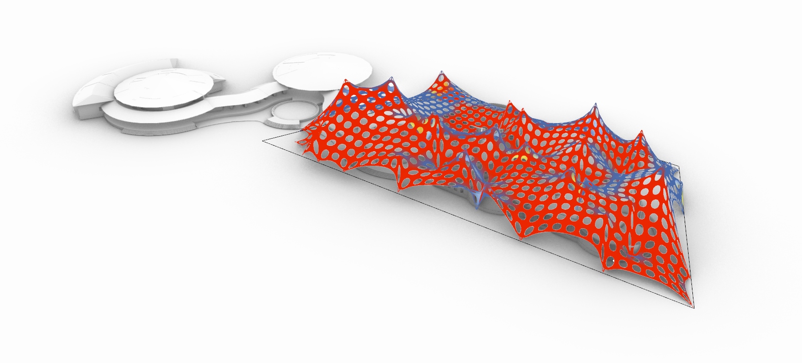
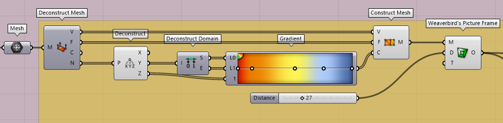
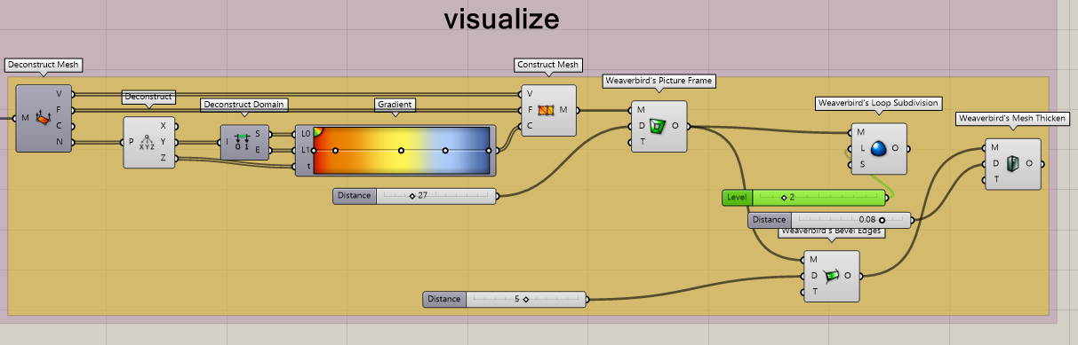
Step 7: Deconstucting, Visualising and Analysing
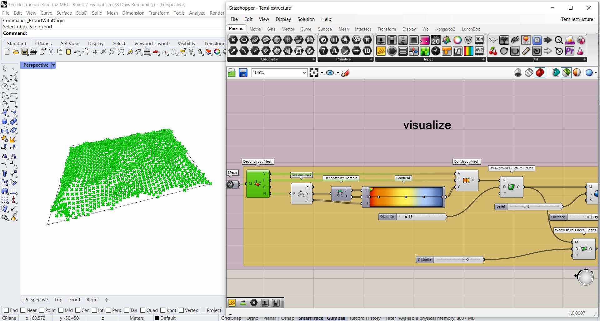
Deconstructing of Mesh for Analysis

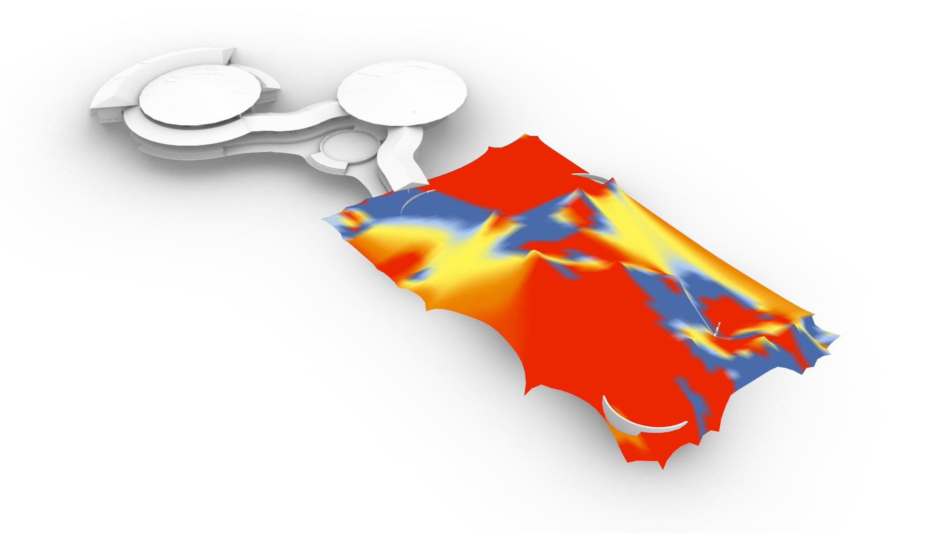
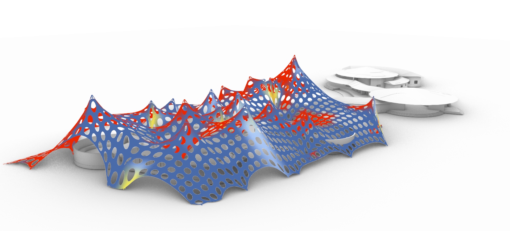
ANALYSIS
The trough and crest of the structure is analysed here. For the same, the mesh is deconstructed first and a Gradient component is used for analysis. Here the Red gradient represents the Crest and the Blue gradient the trough. The Mesh is reconstructed using the Construct Mesh component.
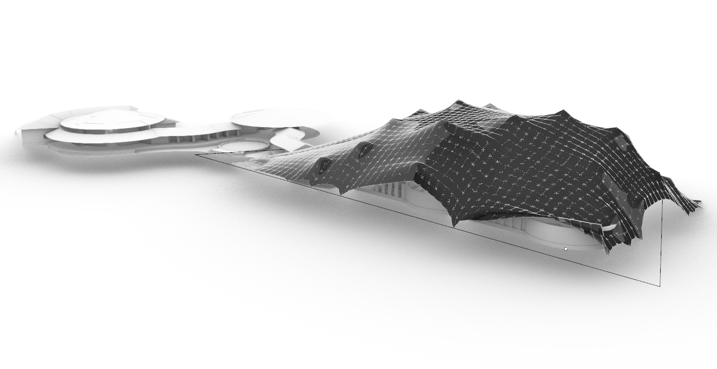
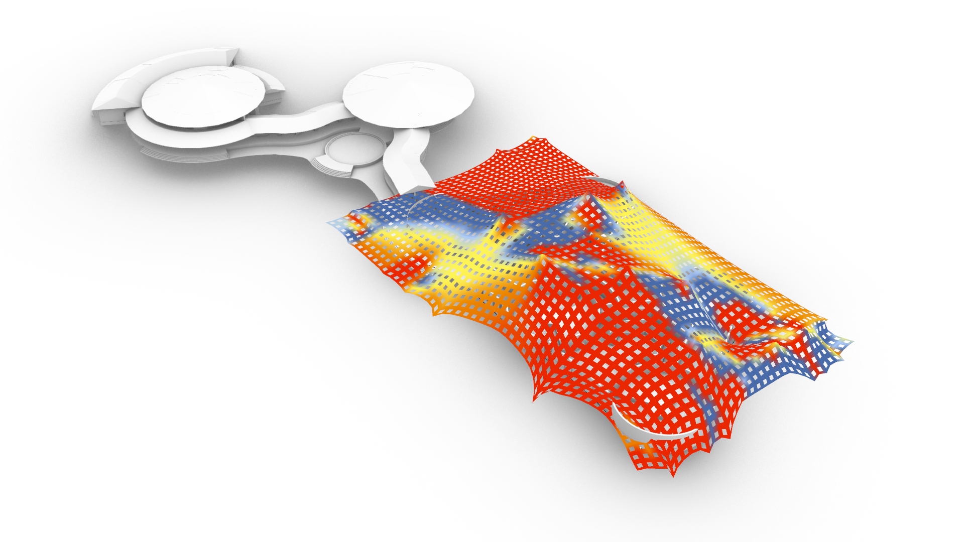
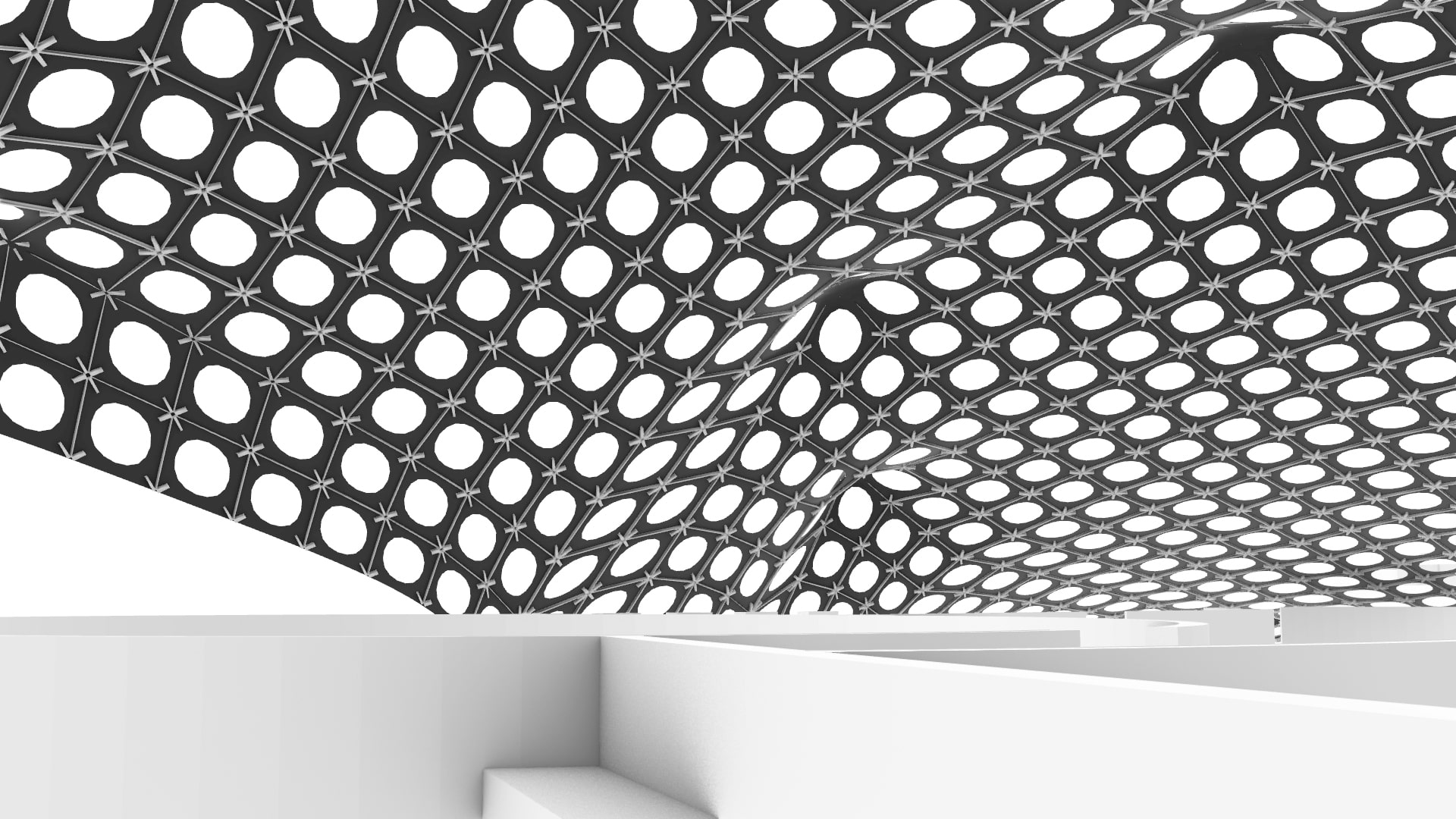
Further the weaver birds tools like Weaverbird Picture frame, Weaverbird Loop Subdivision and Weaverbird Mesh thicken is used to define the perforation size and shape, the mesh support etc.

Weaver bird -Picture frame

Weaverbird loop’s subdivision helps to smoothen the edges of the perforations.

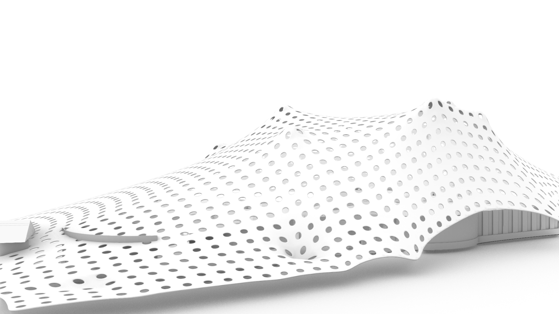
Weaverbird’s mesh thicken gives us an output of a possible frame structure for construction.

Rhino file- Tensilestructure
Grasshopper file- Tensilestructure