B212-500CAD4+555CAD4
Supervisor: Ing. arch. Simon Prokop
Autor: Bc. Tomasz Kloza
The project Micro Micosis is an utopian vision for growing living architecture. A world where buildings and structures arise from the minimum and create far reaching structurally outstanding bodies.
I claim the biggest living organism on Earth – Mycelium – to have that kind of perspective.
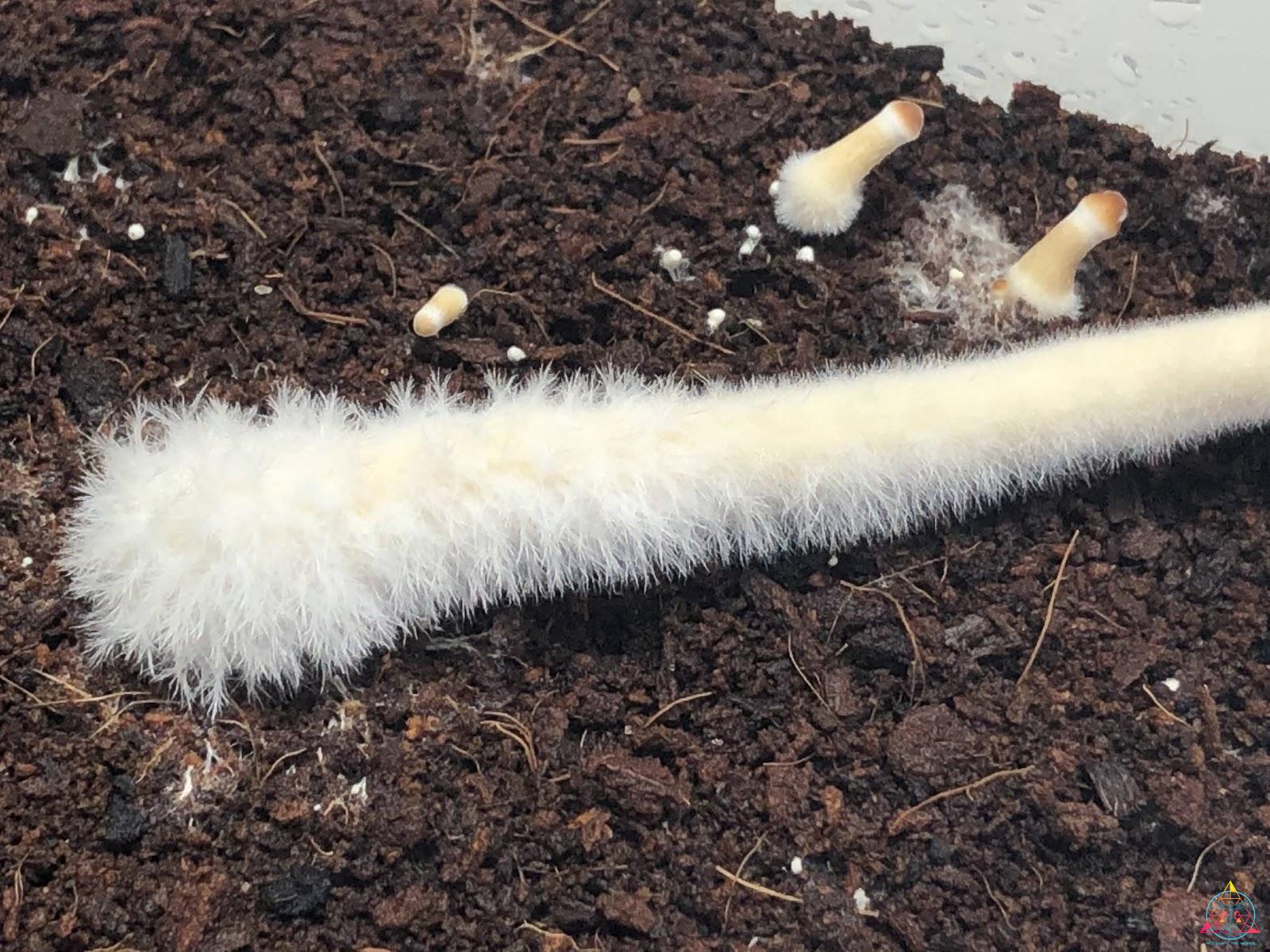
Mycelium is a vegetative part of mushroom growing underground where if finds its nutrition in cellulose and lignin rich substrates or carbon-based organic matter. It creates a network of interconnecting hyphae, serving as information and nutrition exchanging agents. An intelligent being searching for food.
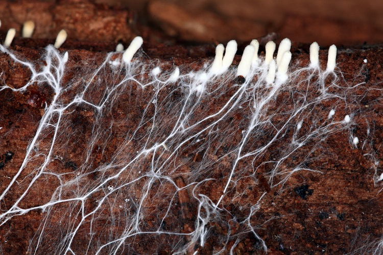
How do we get the Mycelium to grow above the ground and create our desired structures? Have you ever heard of lichens? Lichens are soft of a combination of fungi and algae. The fungi provides a body and shelter for the algae, which by photosynthesizing provides its host with nutrition. Together they form symbiotic lichens. Some mushroom species have been proven to have the ability to be manipulated into endosymbiosis – an artificially introduced symbiosis. This allows for a creation of photosynthetic mycelium. Mycelium naturally scans and explores its environment sometimes even forming aerial mycelium and reaching above the ground. With algae within itself a sun or a source of essential sun-rays could be the growth driver and its media.
Mycelium also is capable of computing. It in no means gonna replace computers, but this ability will allow it to form self-assembling structures. It could be that AI or soft robotics would control the body.
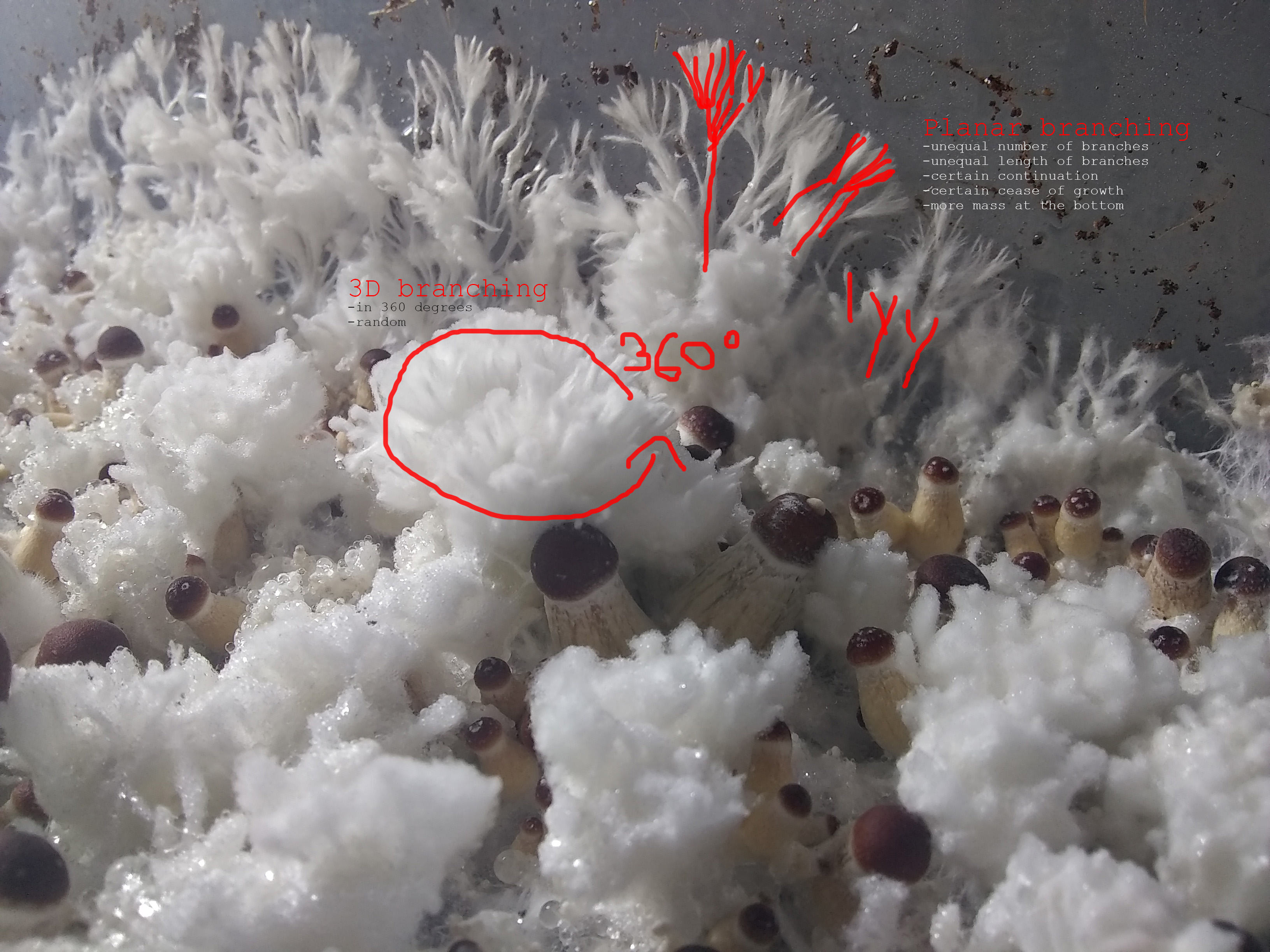
After examining the principle of aerial mycelium growth it has been noted to be fairly similar to L-systems in Grasshopper for Rhino 3D. As that may work more based on fractal-like branching a more random way has been evaluated to be more suitable as hyphae network of mycelium does not grow perfectly equally. A new script had to be develop and it has to be planned as the whole complex.
Steps taken:
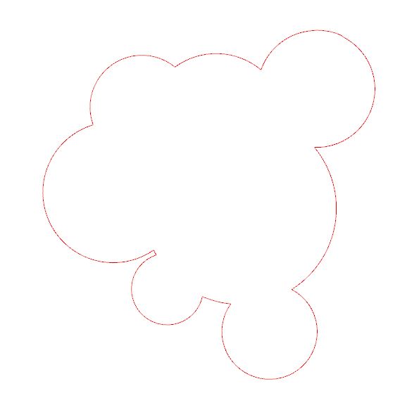
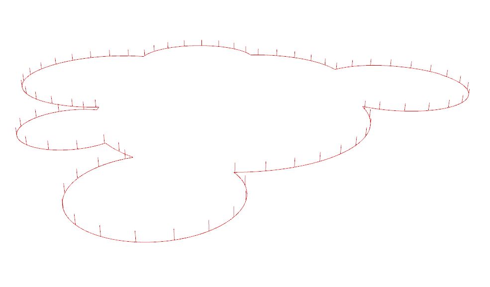
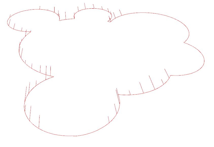
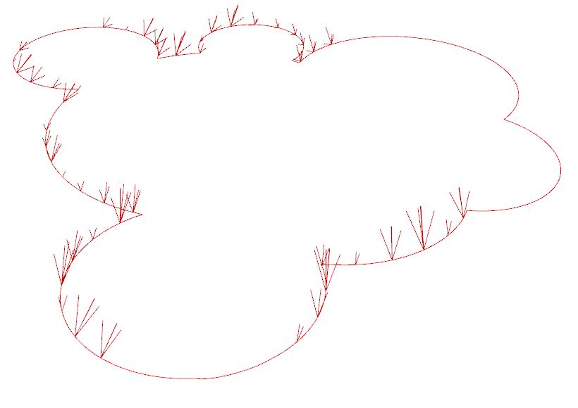
1. Generate a floor plan in a form of Closed Curve. In this example Grasshopper plug-in Termite Nest has been used.
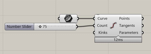
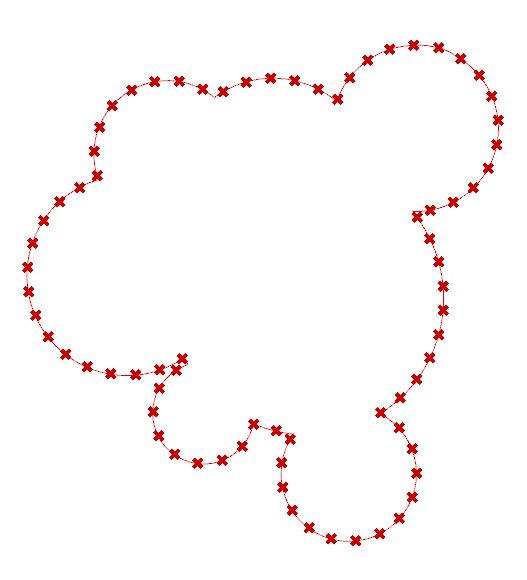
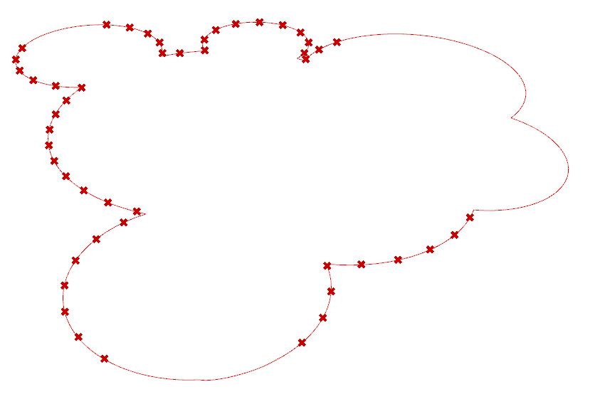
2. Divide the Closed Curve in order to create starting points for individual branching aerial mycelium.
3. As looping with Anemone plug-in will be necessary we need to create the desired input (Data (D0) as tree) generating our design basis. Listed analysis have showed that the algorithm will be based on branching Curves. In order to create the input Curves we need to incorporate into our starting points. We want the geometry to start at [x,y,0] – a planar “Level 0”. As we will be looping our input Curves we will always want to take its End Point in the looping part and branch from there. This indicates us that we need to have the direction of the input Curve in check. Set Number (N) of iterations in Loop Start command as a Panel for conscious choice and a panel for Counter to see the process of the Anemone plug-in and a stage of iteration calculated. Button and Loop End command should always come all together when setting up a looping part of a script. The input Curves are created simply from the starting points. The basic command in Grasshopper is Line SDL needing only one Starting point and direction and length. Direction and length is irrelevant so we will leave its preset to z axis and unit 1 (you may not see them at this scale depending on your modelling environment and Closed Curve floor plan dimensions). With this settings as they are the later extracted input Curve End Point would be located at [x,y,1] and we do not want that. A simple fix is to Flip the input Curve.
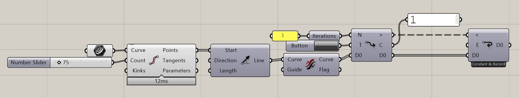
4. Now how do we exactly plan to do the branching? What kind of logic would be behind it? The mycelium and algae endosymbioses embedded intelligence should be the algorithm design driver. Photosynthesizing organisms do reach to the sun and guide and alter their growth according to the sun-rays affected environment. The scripted geometry has to have a simulation of the sun. As we only aim for sort of a ‘prototype’ it is acceptable to use a dull uninformed element placed manually. We want our scripted aerial mycelium to grow towards the exemplar sun source. To illustrate more random and irregular behavior in nature we will not set it as a point, but rather a random or semi-random points embedded at manually placed surface. Ideally perhaps an exact sun path, intensity and growth fluctuations would be contained in the informed algorithm, but for these we do not have either empirical or theoretical data.
5. We set the randomness factor by generating one Point from the mimicry of sun Surface bounds using Populate Geometry with 1 Count. To ensure a different point will be generated with each iteration of the looping Anemone we will use Counter output from Loop Start as a Seed in our Populate Geometry command as it gives the exact number or current iteration processed which does not repeat in the process.
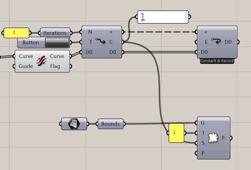

6. Living organisms tend to sacrifice parts of their body in order to ensure its thriving. Size of the can be body adjusted according to how much nutrition is available in order to sustain organism’s demand. Unproductive parts without potential have no reason in continuing to grow in contrast to the highly efficient ones being the providers. In this script we work with curves in our Anemone algorithm, but as nature and as mycelium we should be selective of which agents will continue to grow and which will cease their immediate continuation. To do that in Grasshopper we take the looped Curves, find their count using List Length and via percentual elimination by Multiplication command. After this process we are left with a number that we need to use in input Count of Closets Points command to retrieve the closest most prospering curves reaching to the simulated sun, respectively their end point as that’s the matter for the building of next algorithm steps.
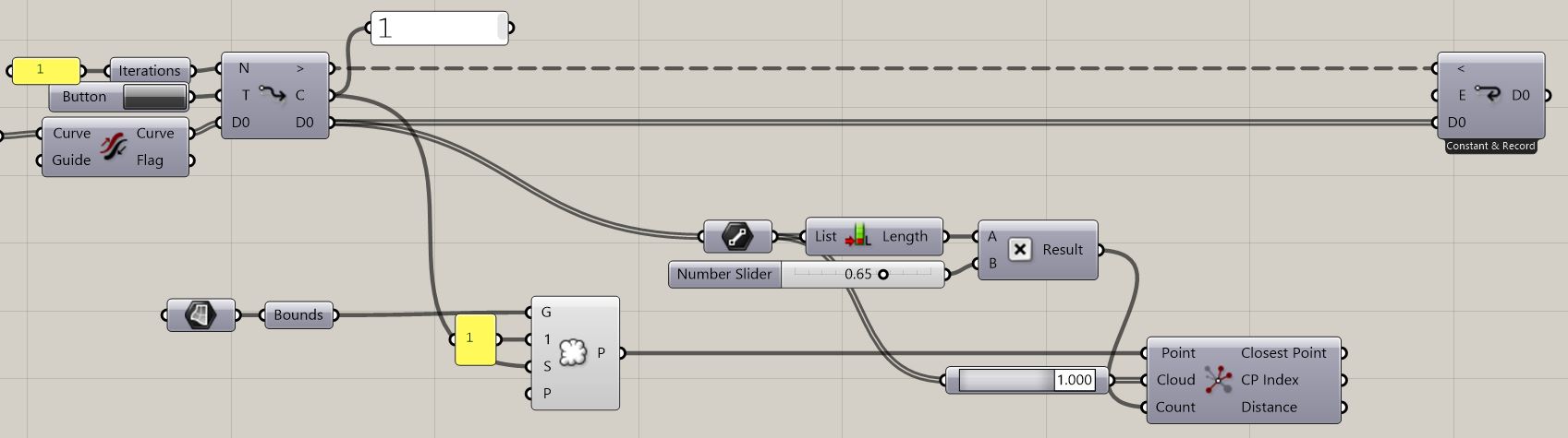
7. We will be creating simple curves (lines) using Line SDL command. We have the selected points that we want to use as a Start, Direction as a Vector 2pt going towards the sun from individual points and in order to mimic nature rather asymmetric growth we will script it again in a dull unfounded way using randomness aspect in our design of Length. Random command operates on our defined and controlled domain. Number or generated random values within the given domain and number of data for Line SDL have to match. To further add onto the randomness aspect of things we can use Counter as a Seed for our Random command.
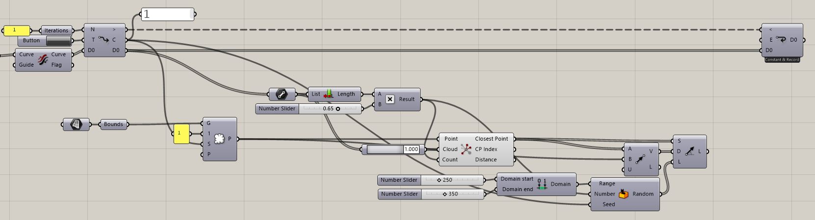
8. Now to mimicking the actual branching system. We want our looped Curves to follow the direction of the sun-rays, but not to create a complete straight line. This is not how mycelium behaves according to our analyses. It is aware of the direction, but branches out in a continuous search for exploration. Therefor, we need to have a 3D system of semi-controlled branching. To do that we take a Curve that is aware of the direction using a 2pt Vector command. An easy way to branch it in informed way is to create a Perpendicular Frame at the end of that Curve and Deconstruct Plane of the generated Frame and Construct Plane out of x-axis or y-axis and the Vector of our simulated Sun-rays reaching the mycelium in such a way that later we are able to Rotate the objects in a plane. This first step rotation will randomly tilt from the original path in a semi-controlled manner by using Random command with defined desired Domain to generate varying Angles and a Counter as a Seed for previously mentioned effects. As we desire again to step up the randomness lets also randomly within a controlled and desired domain dictate the number of branches created via additional Random command for number of branches ruling the Number of random values generated for the Angles. A need for grafting is necessary in the Rotate command to match the data tree structures.
Please note that at this point it is highly recommended to check the attached grasshopper script as the algorithm connections created in this part are very parametrically sensitive.
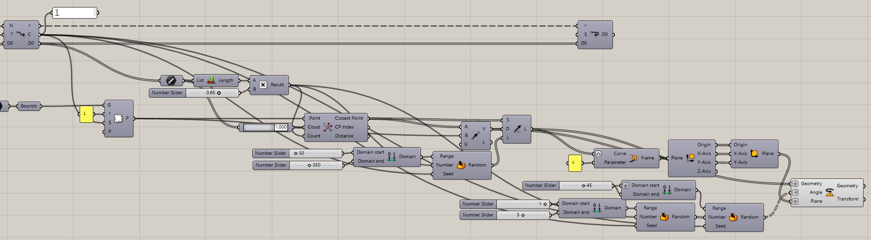
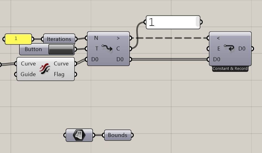
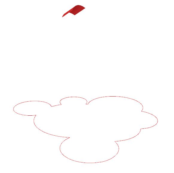
9. So far we have achieved a planar branching. Now in step two of ensuring a 3D branching logic we need to use a 3D Rotate command. Here again we have to have our continuous subsequent curves system ensured by properly managing the Center input being the end of the previously looped curve. Again we semi-control the Domain of randomness and select the direction aware curve as our Axis for Rotate 3D command. Flattened output is now being ready for more iterations in our Anemone looping script. Do not forget to set Loop End to Record Data by right-clicking it and choosing the option. It will be necessary for the final step to have all generated curves all together.
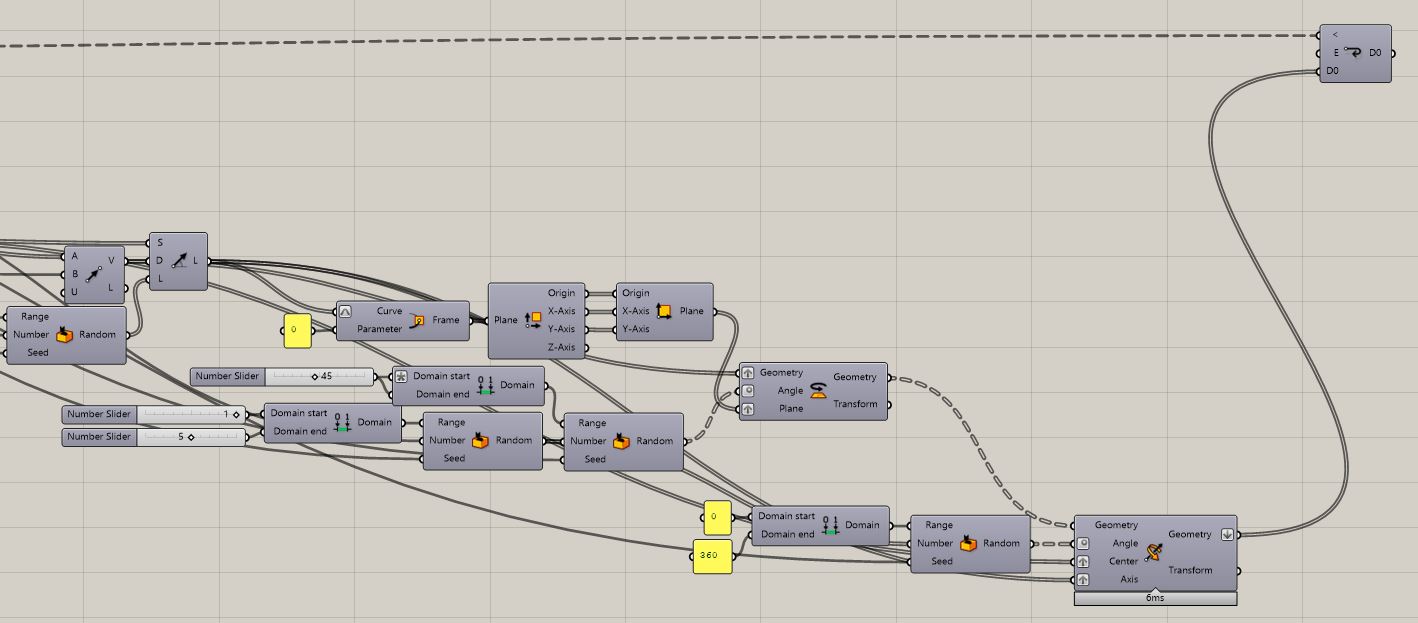
10. We will not be stopping at branched curves as we want to give them some sort of mass. For turning curves into meshed mass we will use a Grasshopper plug-in called Dendro. As with every single iteration Loop End will output new developed data it is unnecessary to us for Dendro to generate meshed mass with every iteration. It would be heavy for the software computing abilities. In situations like this when we are not required to see every iteration in its final form we can use Data Dam to control the data flow in our script. Do flatten the outcome curves from Loop End as we do not want to work with data trees made of groups, but we want to access individual elements. We now can play with the Dendro plug-in by setting up the basics first like Curve To Volume component and its required input Create Settings. For Curve Radius input we can set a constant value or play with the Remapping and Graph Mappers. Only note that Voxel Size should not be more than one third of given smallest Curve Radius value to ensure proper functioning of the Curve To Volume component. For the maximum value given to Curve Radius in our example we will calculate the length of the floor plan Closed Curve and divide the result by our Divide Curve Count input to get the exact length of the segments generated by us at the beginning. As we talk about radius we need to further dividing it by 2 before feeding it into the desired input.
Please not that Remap+ component I have in my script is a Cluster and you can access its inner algorithm via opening it if you with to inspect it.


You will end up having a lot of Curves for Dendro in the end of many iterations to process with current setting. It is advised to selectively continue using List Item component or any other workflow.
Note that variations in any or all inputs can change the structure significantly. It is up to you to experiment and test to achieve your desired outcome.
Do continuously name and group your script. Use panels for values that are constant. Use Scribble command to ease the orientation within the script. The provided attached algorithm is being left clean and unmarked and left for your preferences adjustments.
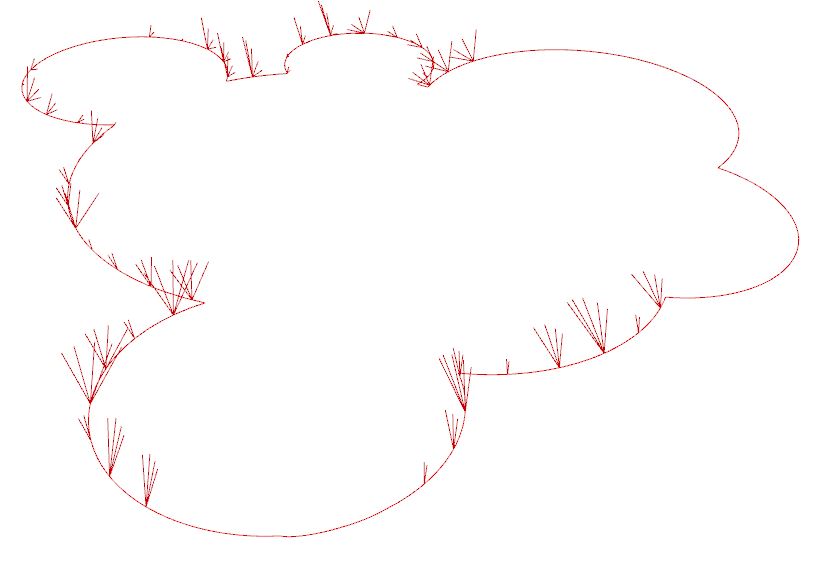
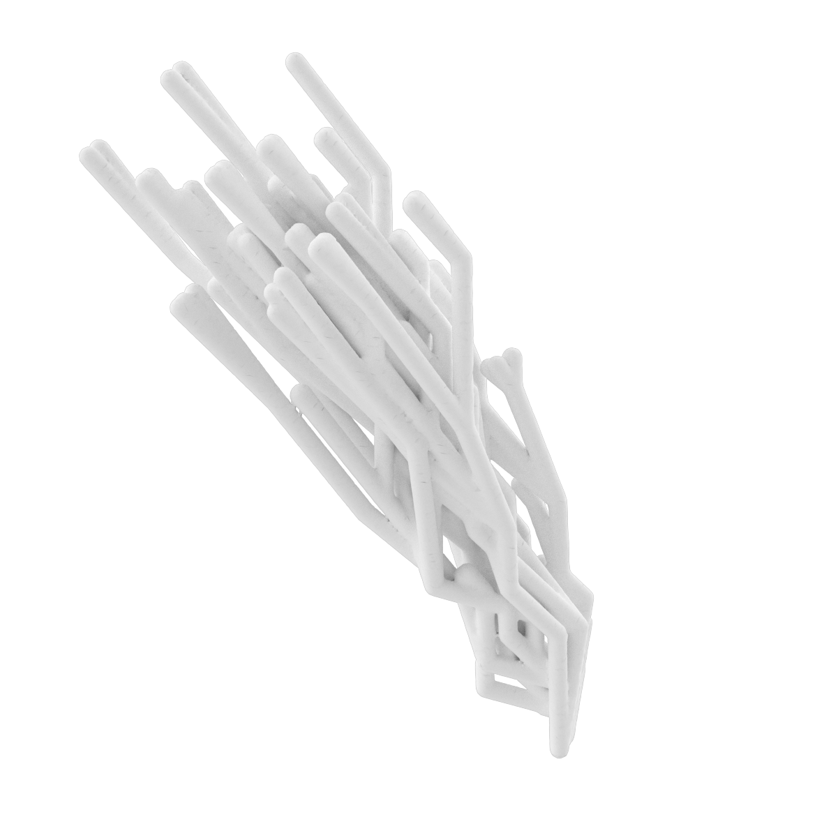
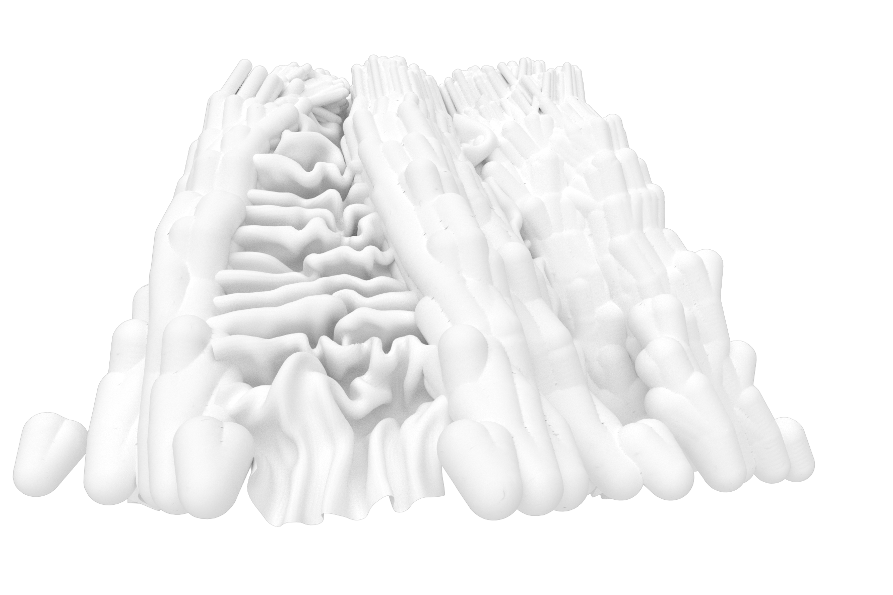
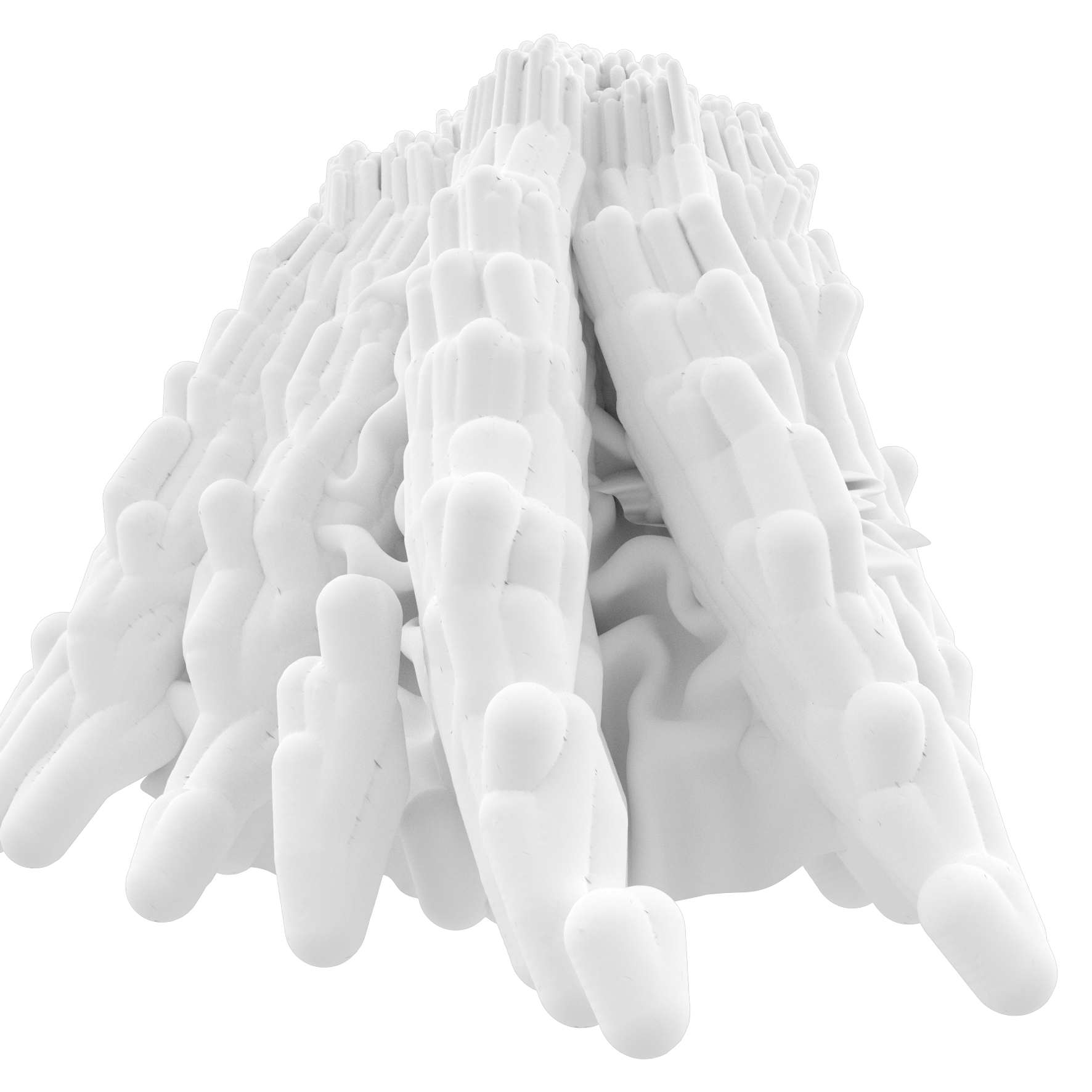
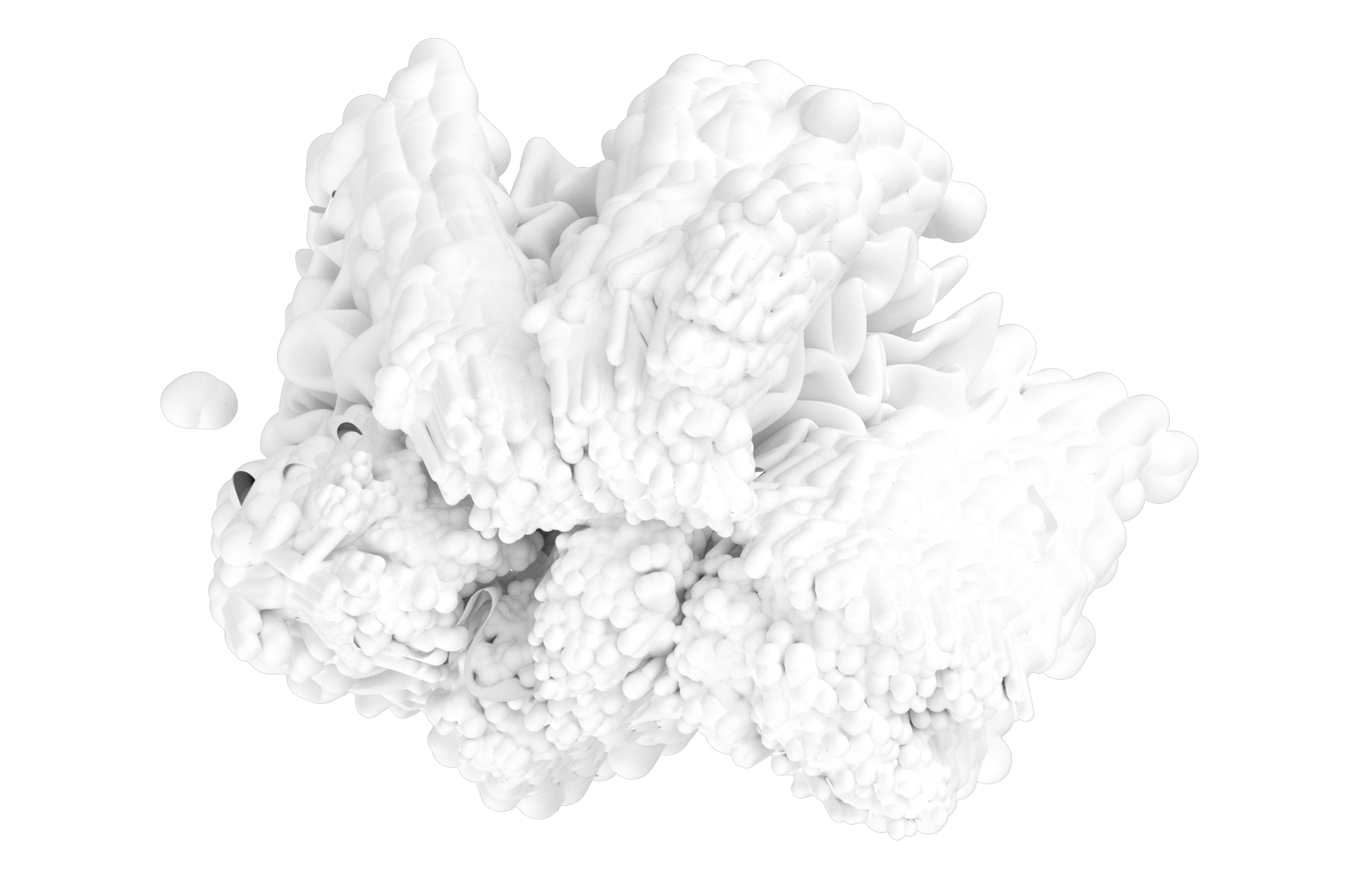
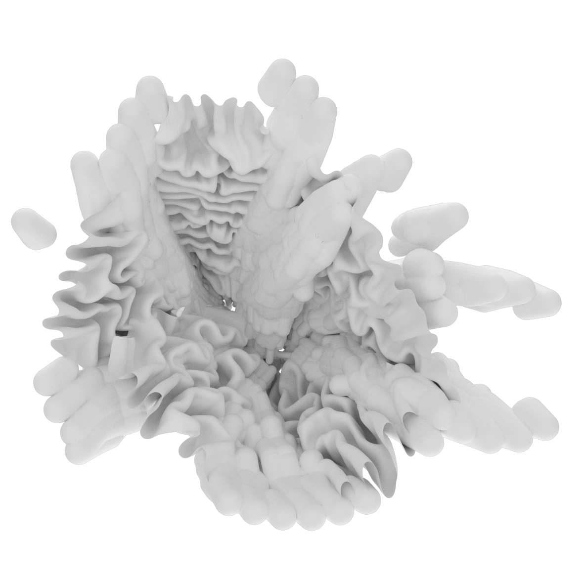
Below is a list of single branch options that you are able to generate:
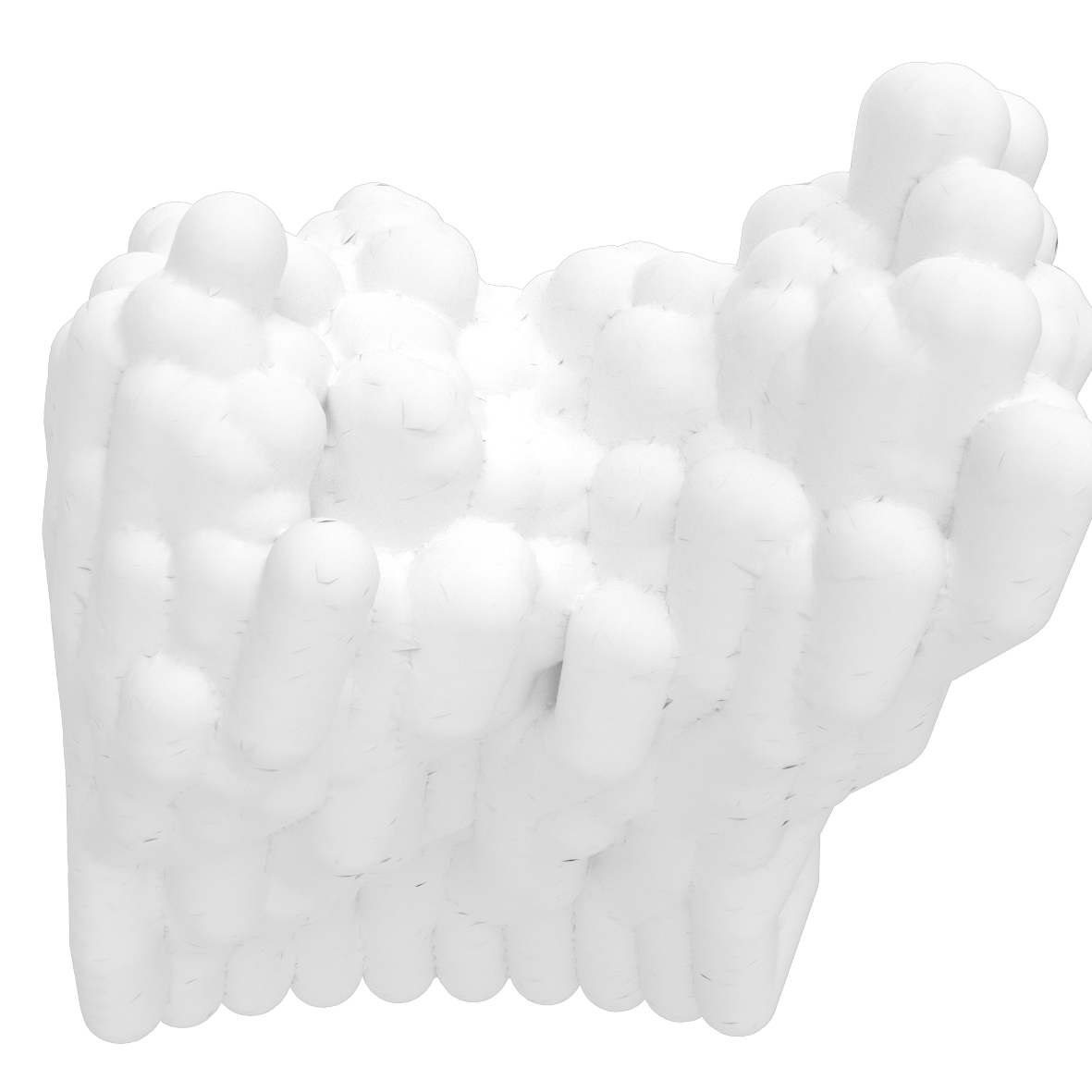
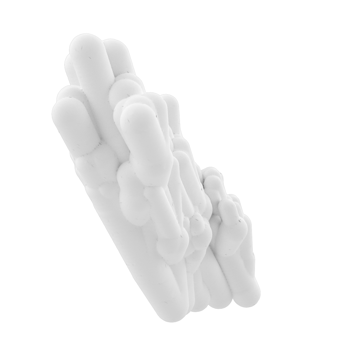
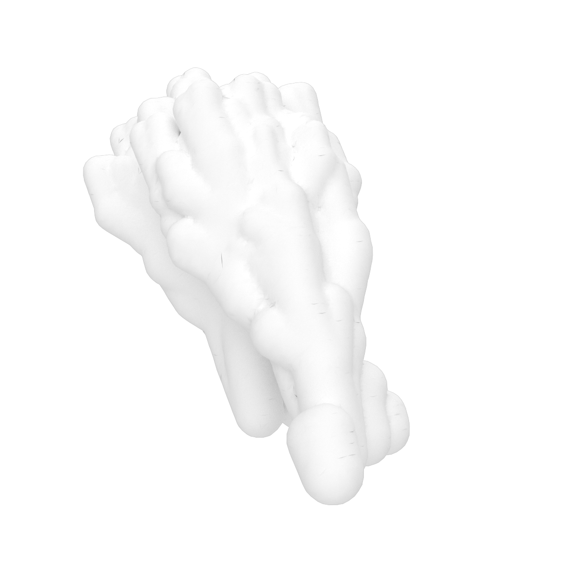
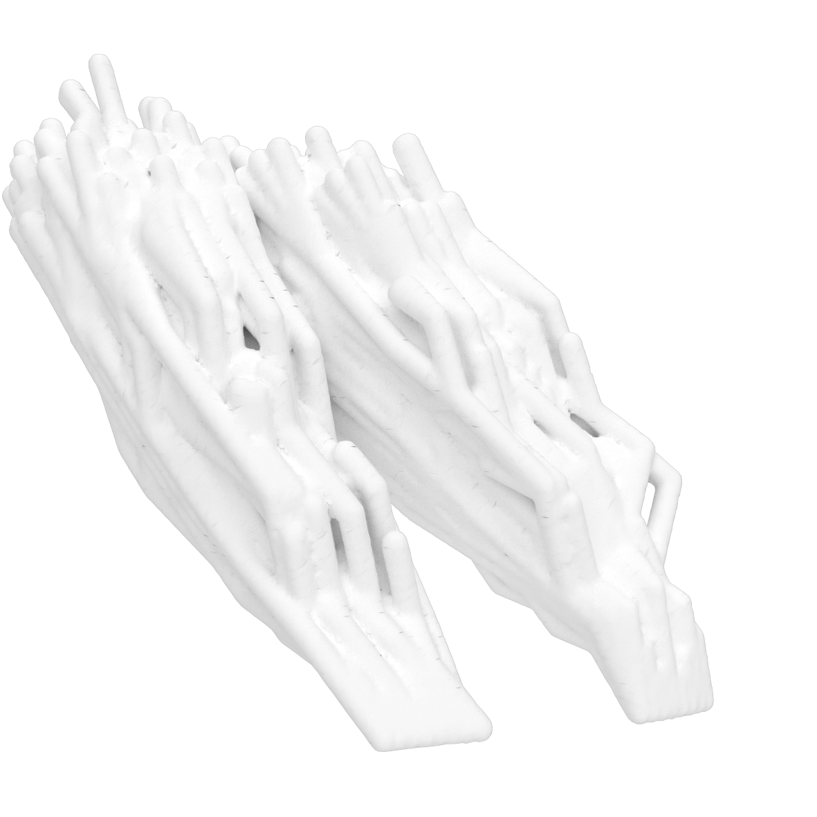
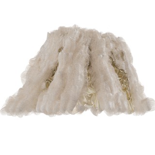
The final outcome using the last listed single branch parametric settings:
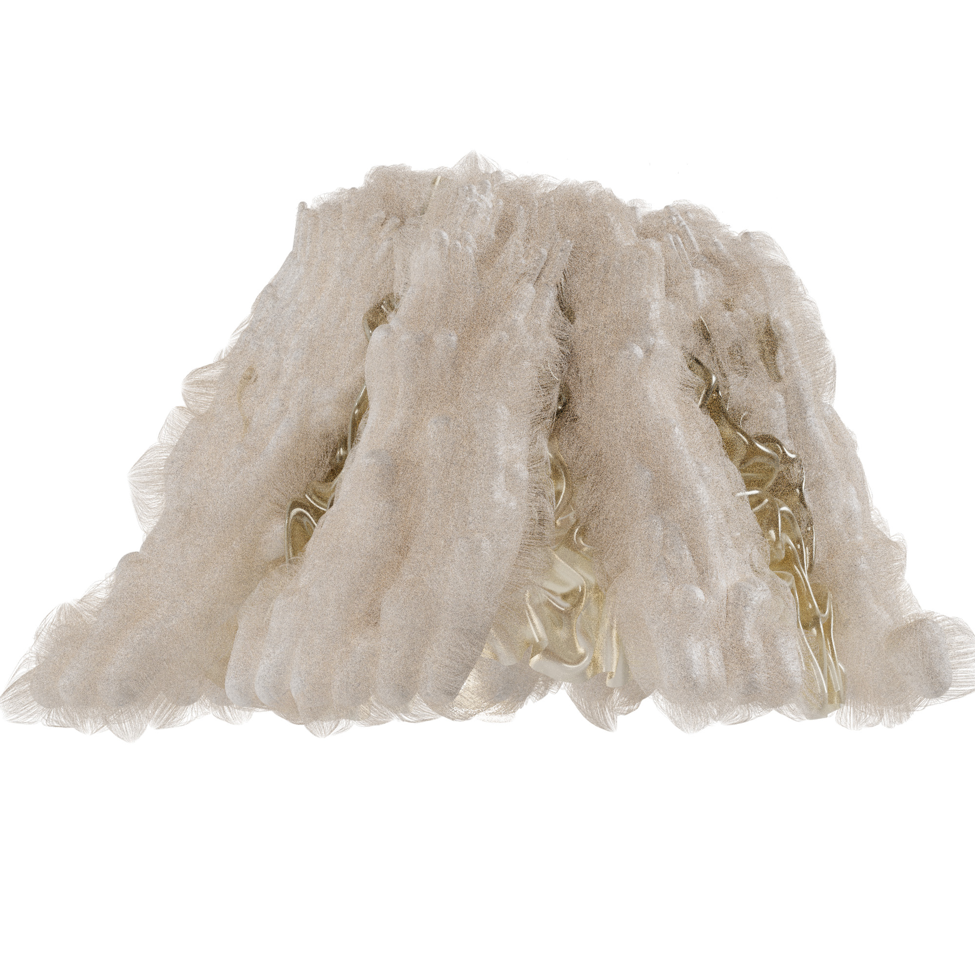
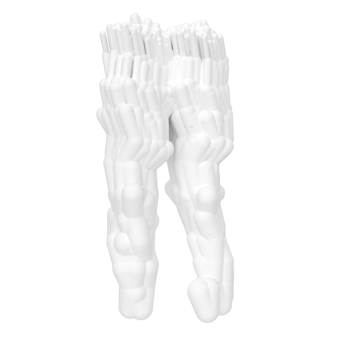
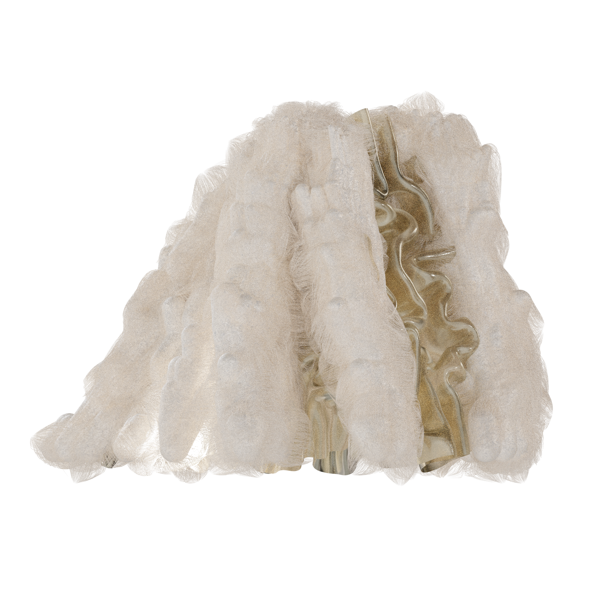
The final outcome after processing it with Blender materials and Hair effect:

Resulting Grasshopper script:
B212-500CAD4+555CAD4_Micro Mycosis_Bc. Tomasz Kloza
Closed Curve generated Floor Plan and Surface as Mimicked source are internalized as the final Rhino 3D model exceeds uploadable size.