Parametric Facade Parametric Facade
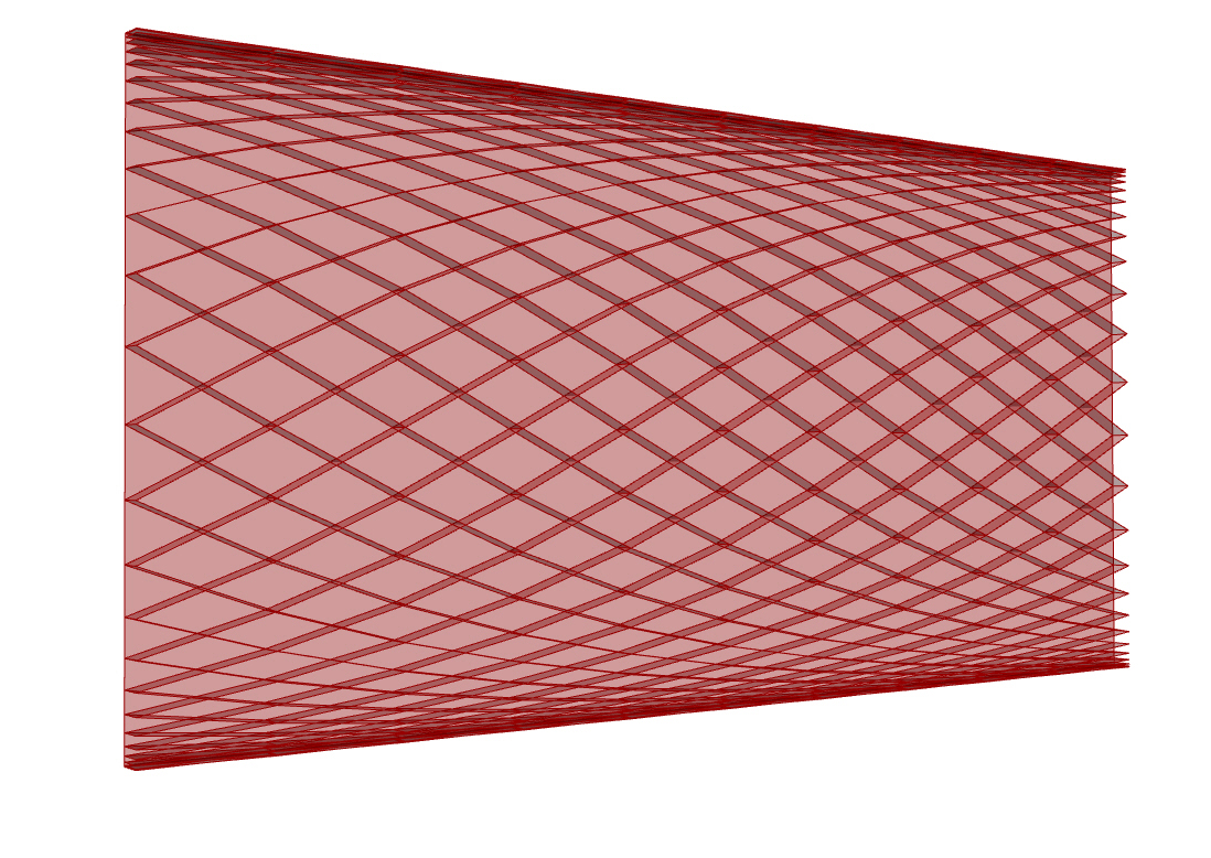
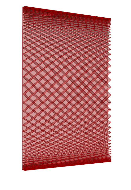
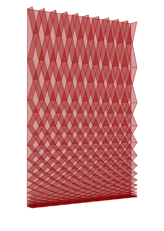
The goal was to create a parametric facade that can be easily modified in order to adapt it to the variations of the building or to use it in completely different projects. The versatile parameters should include the dimensions of the facade, the form of the grid, its density and its depth. By these variations one can study how the light enters the building, how it looks from the outside, which is the optimal scale of the facade in relationship with the rest of the construction, and many other useful conditions. I chose this topic because it could be actually useful for me. I can easily imagine myself using this model in the next years.
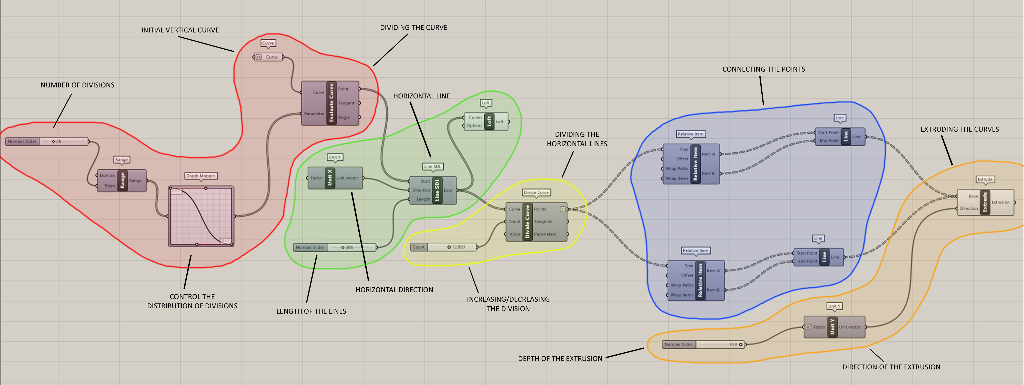
Full script:
Step 1: Initial curve
The first step is to create a vertical line in Rhinoceros that will serve as the base for the development of the facade. We must associate this curve to a “curve” Grasshopper parameter. This will be the starting point of our project.
After this, we have to divide this line by introducing some points along it. We can do this division with the “evaluate curve” function. In this box, we connect “parameter” with a Graph Mapper box. With this option we will be able to control the distribution of the divisions of the vertical curve. In the end, this will determine the form of the real curves of the facade.
By adding a “range” component and a number slider to it, we can also control how many divisions we apply to the curve. This means we can control the number of horizontal curves in the facade; its “density”.

Step 2: Horizontal lines
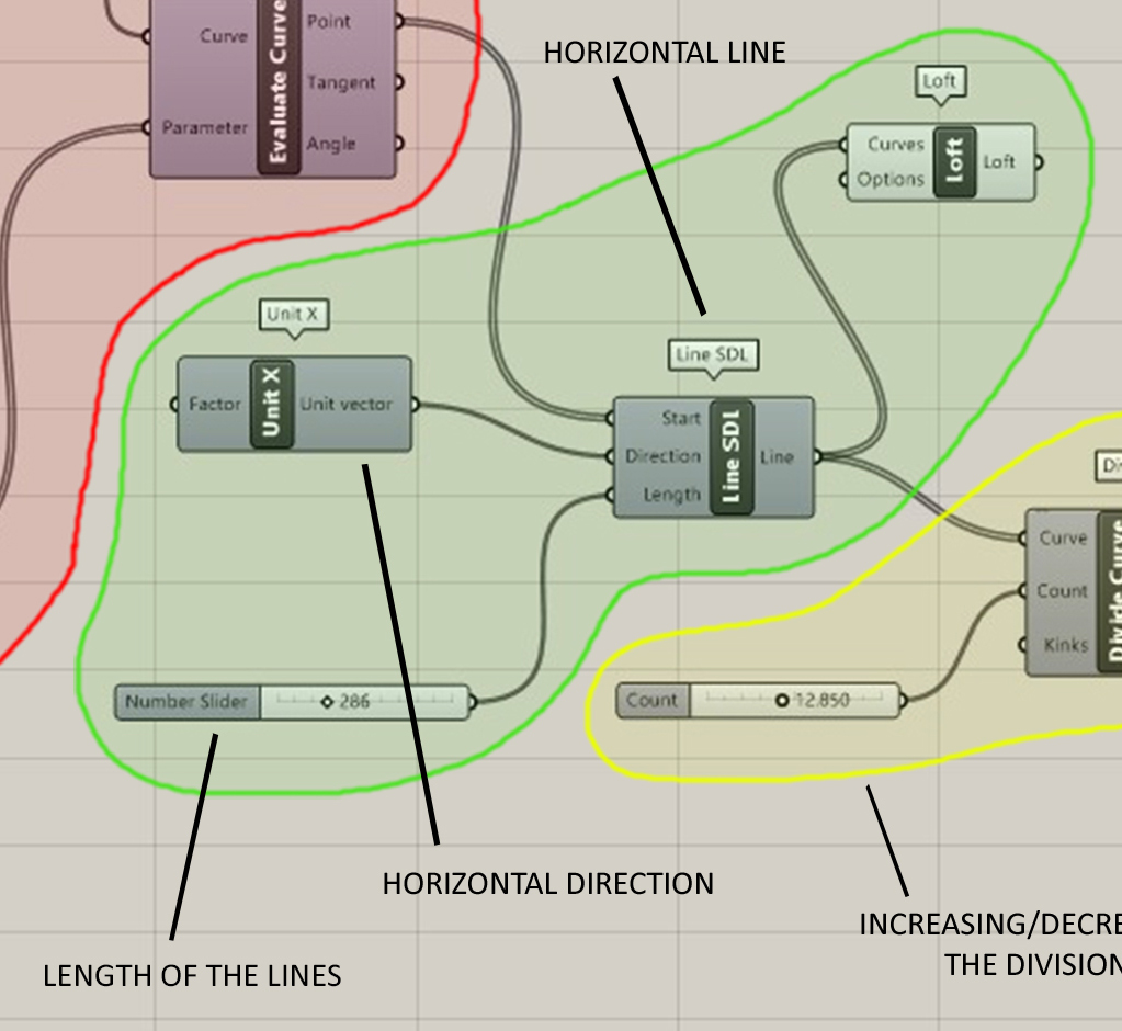
Secondly, we will introduce horizontal lines that start from the divisor points we have already created in the vertical line. We use a “Line DSL” component and connect it to “Evaluate curve”. We have to use “Unit X” to determine the horizontal direction of the lines, and add a number slider to control the length of these lines. Finally, we add a “Loft” command.
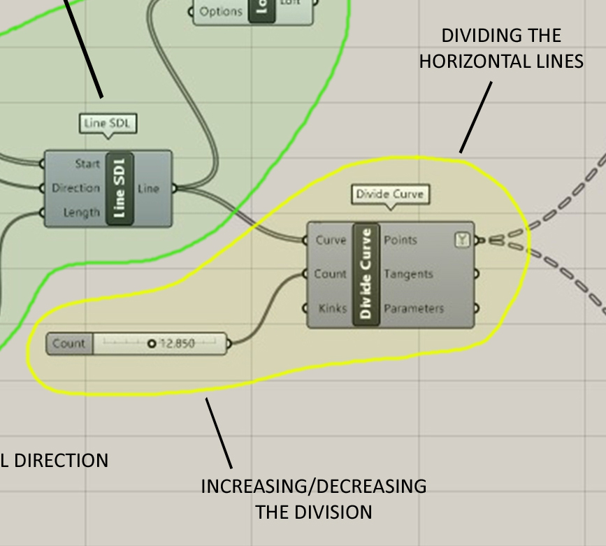
Step 3: Divide the horizontal lines
The third step is to divide the horizontal curves we have just created. W will use the “divide curve” component, connecting it to the “Line SDL” one and adding a Number Slider to it. With this slider we can control the number of divisions. This means we will control the number of vertical curves of the facade.
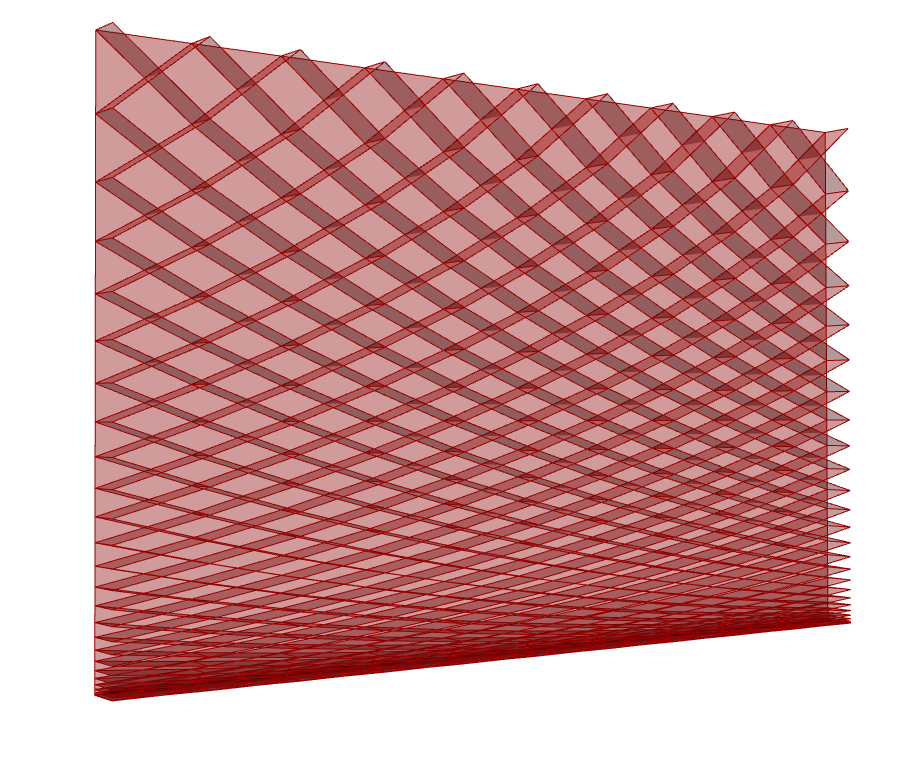
Step 4: Connecting the points
At this point we have created a net of points that are located in the intersections of “imaginary” horizontal and vertical lines. We can modify the number and distribution of this imaginary lines. Now we have to connect these points. These connections will be the “real” curves that will constitute the real facade.
In order to do this, we will use two “Relative Item” commands, both connected to a “line” item. These will be the “real” lines. We have to do this twice because the facade will be composed by two groups of lines, more or less “diagonal” curves, more or less “perpendicular” between them.
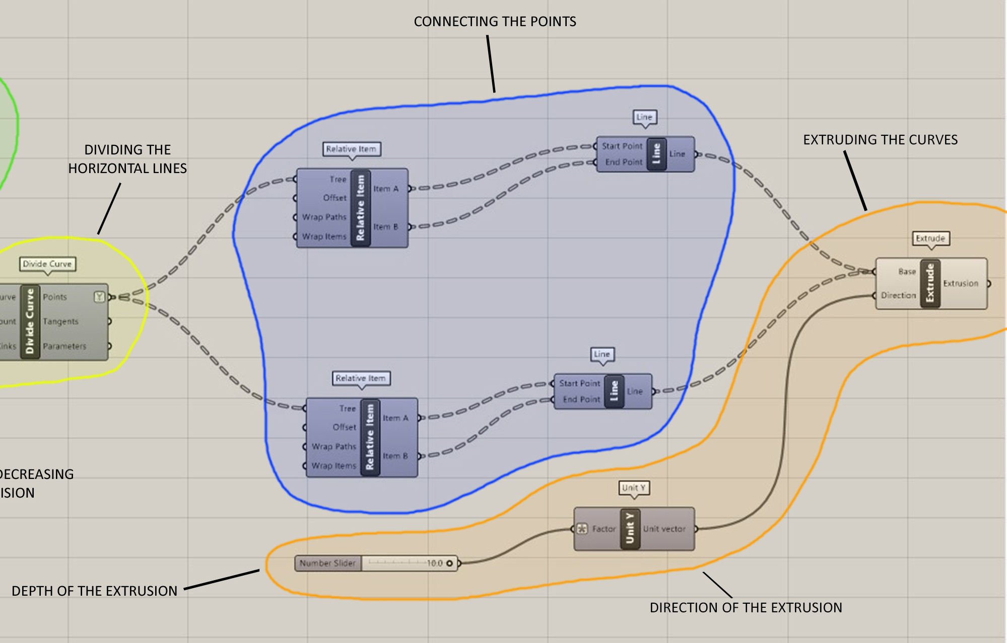
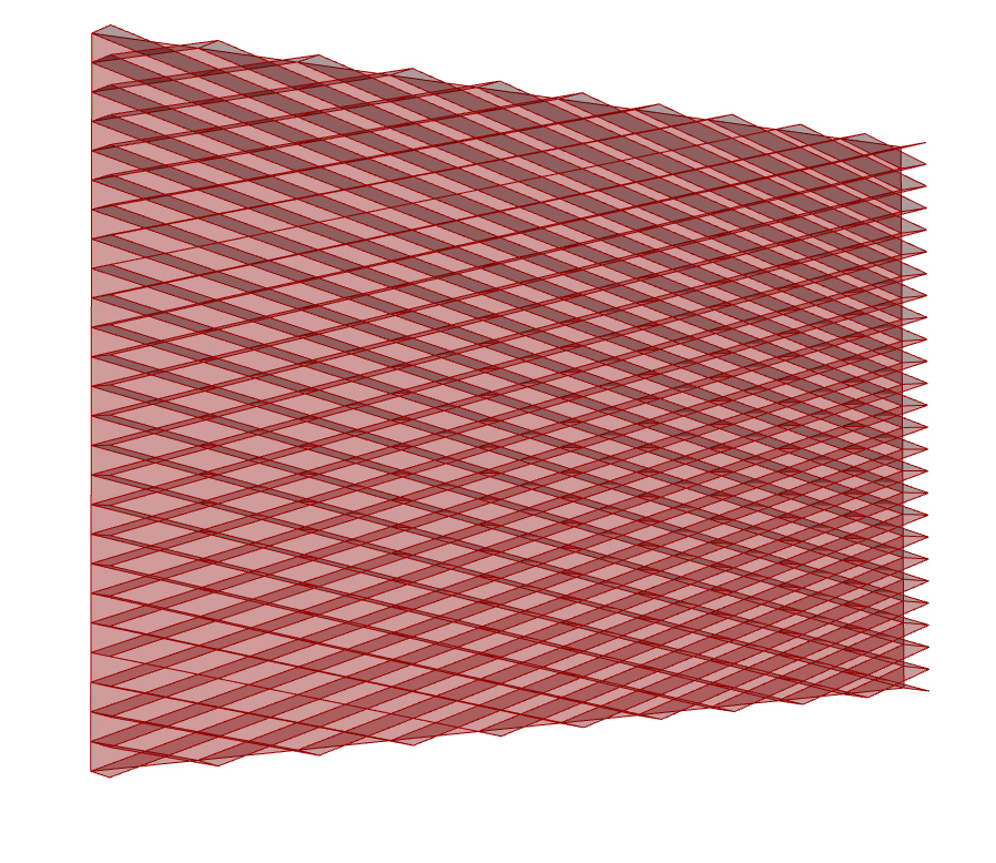
Step 5: Extrude the curves
At this point we already have the real lines that form the facade. The final step is to extrude them in order to give thickness to the facade. We have to use an “Extrude” item. To control the direction of the extrusion we need to use an “Unit Y” item and connect it to a Number Slider to determine the length of the extrusion.