Following tutorial concept allows to create vast modifications of randomization between two types of geometries also affected by an attractor field (parametrical field that affects geometries according to the distance between its focus and the geometries).
It is possible to change the amount of randomization, define the focus of the attractor field and its strength, the amount of each geometries, and of course the type of geometry or initial grid also.
The tutorial is divided into individual sections explained always separately and with relation to others, so you can understand the basic principles, and be able to change it for your requirements eventually.
Tutorial is available at this link:
Tutorial
The Script is available at this link:
Facade design script_1
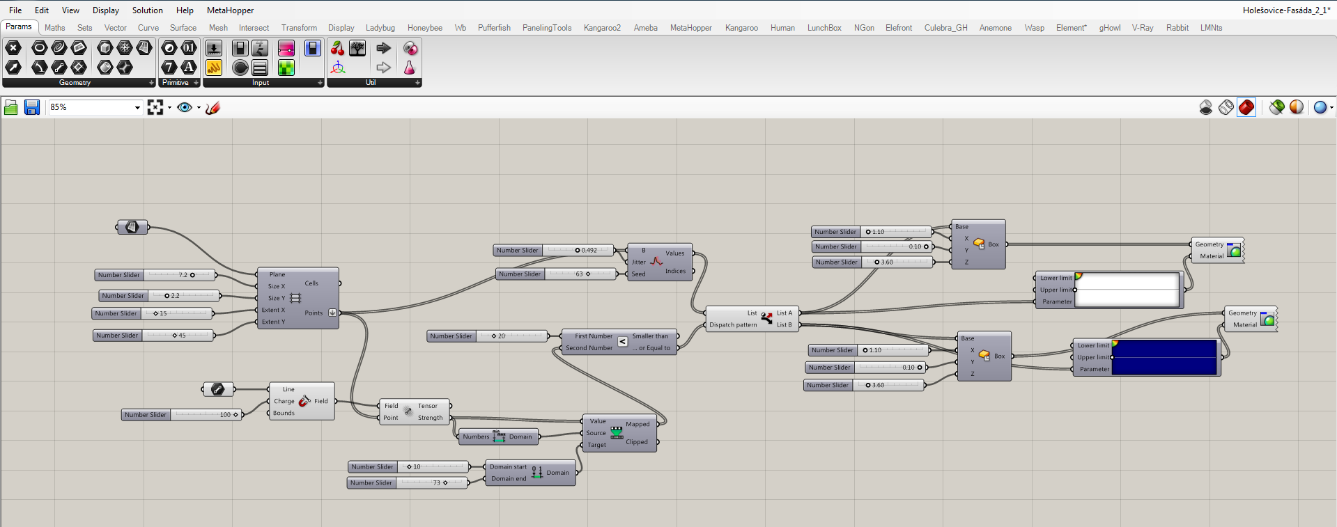
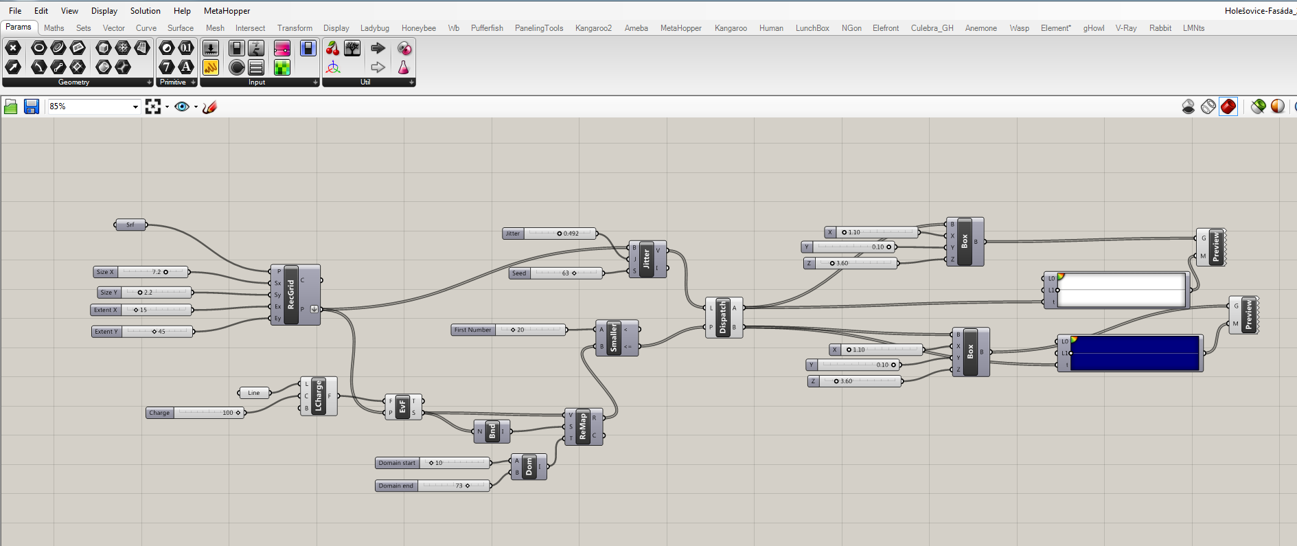
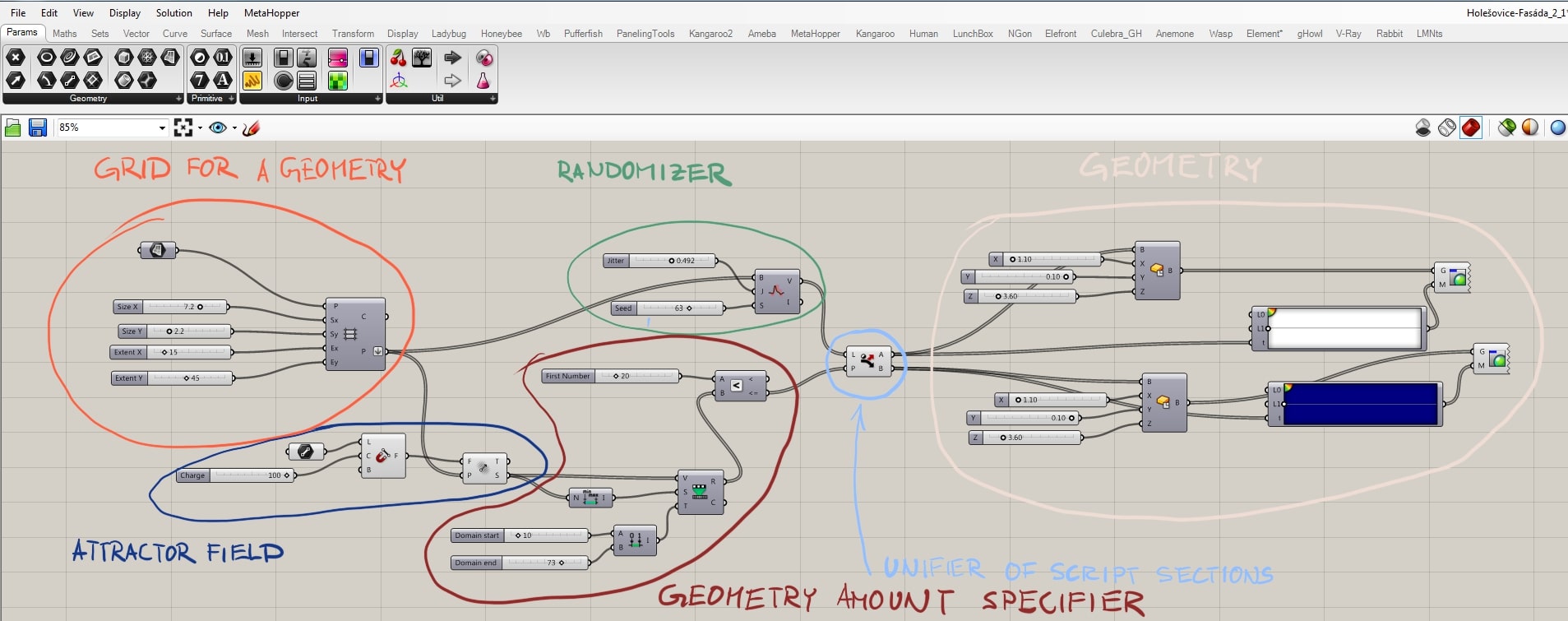
- Grid for a geometry
- You can define initial plane, type of grid, and its parameters
- In this case, rectangular grid was used
- Randomizer
- Part of the script, where the list of grid points are being mixed
- Attractor field
- Defines what kind of geometry would be used as an attractor (line, point, plane, etc.)
- Creates an attractor field defined by the relation of grid points and mentioned geometry
- Geometry amount specifier
- Since I’ve chosen to mix two type of geometries, it is convenient to be able to define the amount of each one
- Unifier of script sections
- Here the randomizer, attractor field, and the amount of geometry are being unified
- Geometries itself
- Whichever type of geometry is technically possible to be implemented
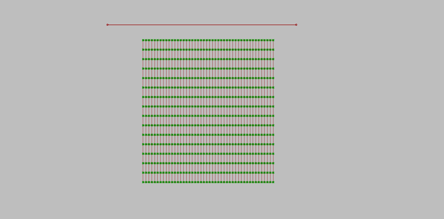
At first, we have to understand the relation between the grid and placed geometry. Following picture shows the grid itself.
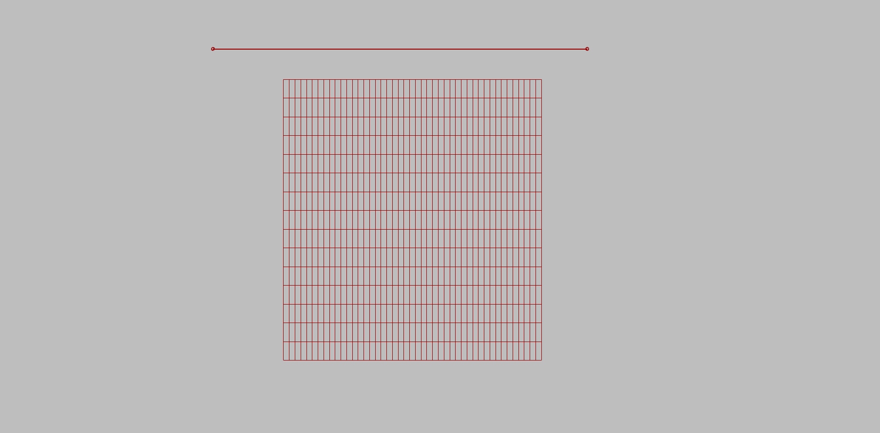
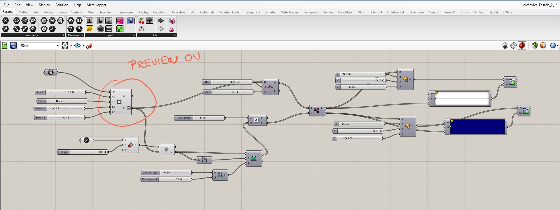
When we put on the preview of the Dispatch component, we can see the center point of geometries.
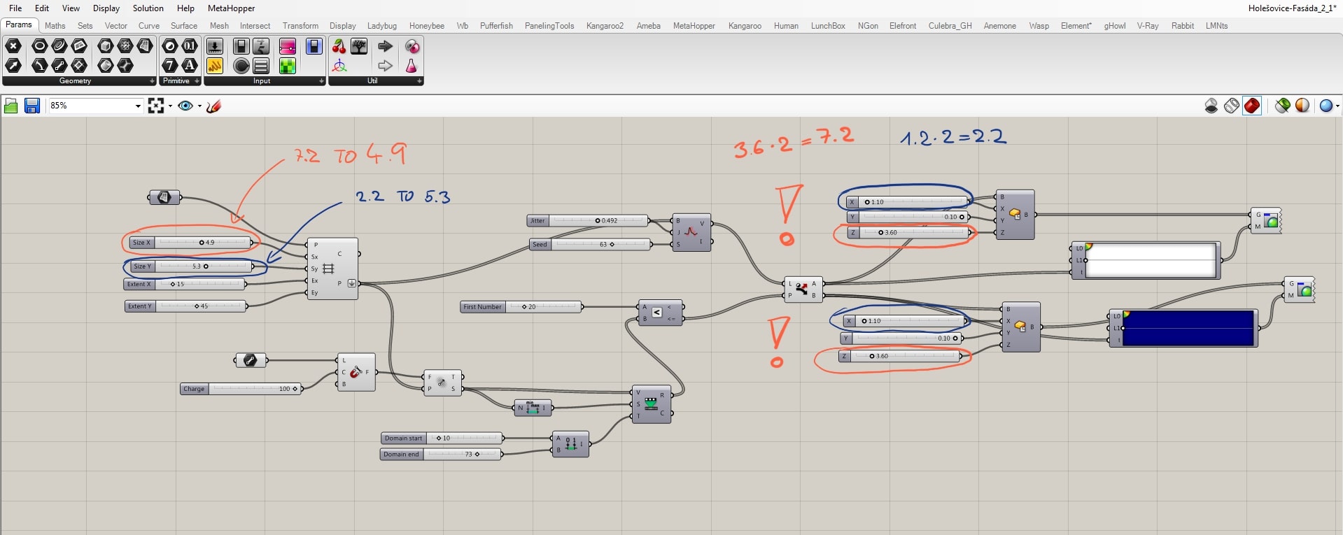
Now it is important to see how the placement of a geometry, size of it and parameters of the grid work together. Changing of “Y” value of the grid increases horizontal distances.
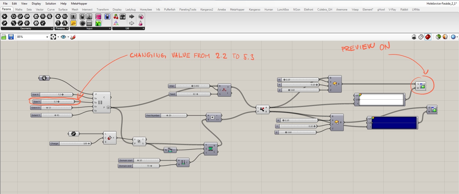
Changing of “X” values increases the vertical distances.
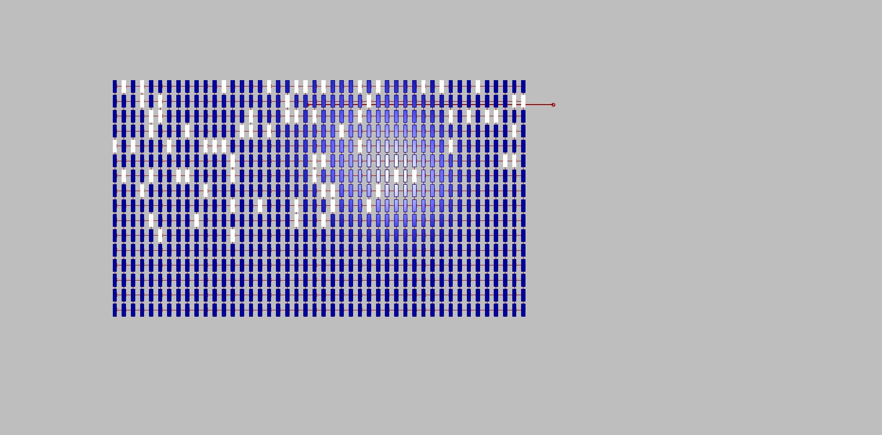
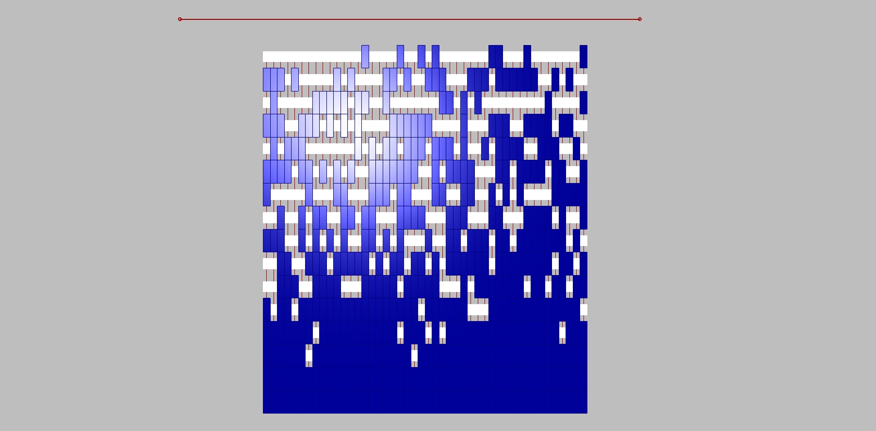
Be aware that in order to have the same size of the grid together with boxes as the geometry, sizes must be in a certain ratio. In this case, the size of the grid equals double size of the box. If you not follow this rule, you may end up with overlapping geometries, as you can see in the picture below.
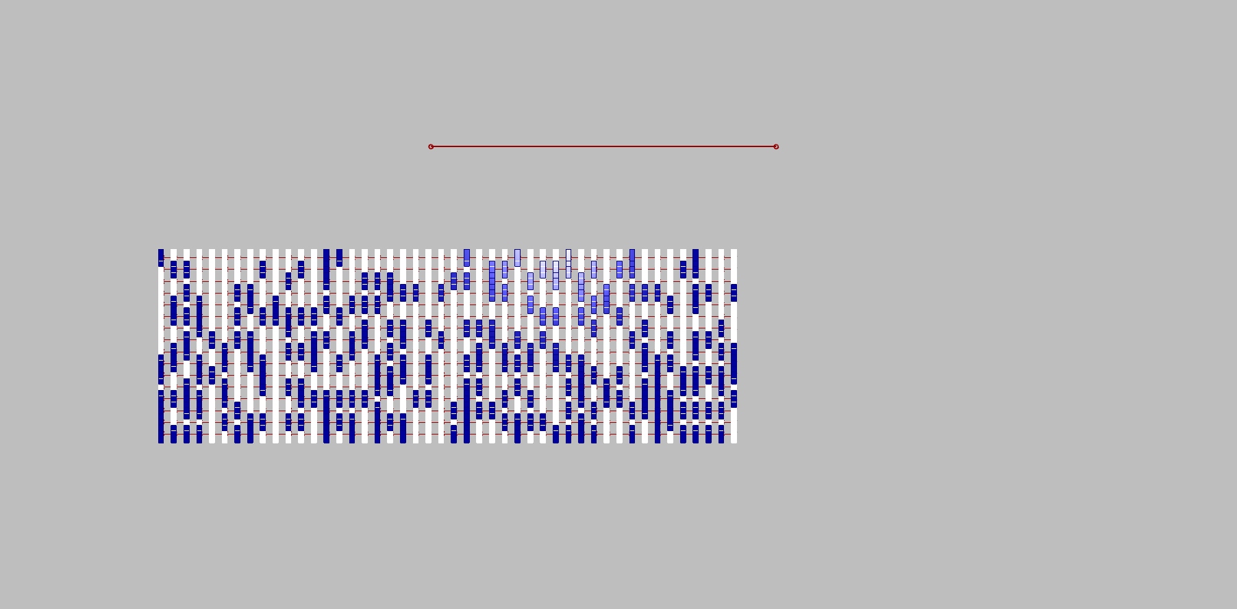
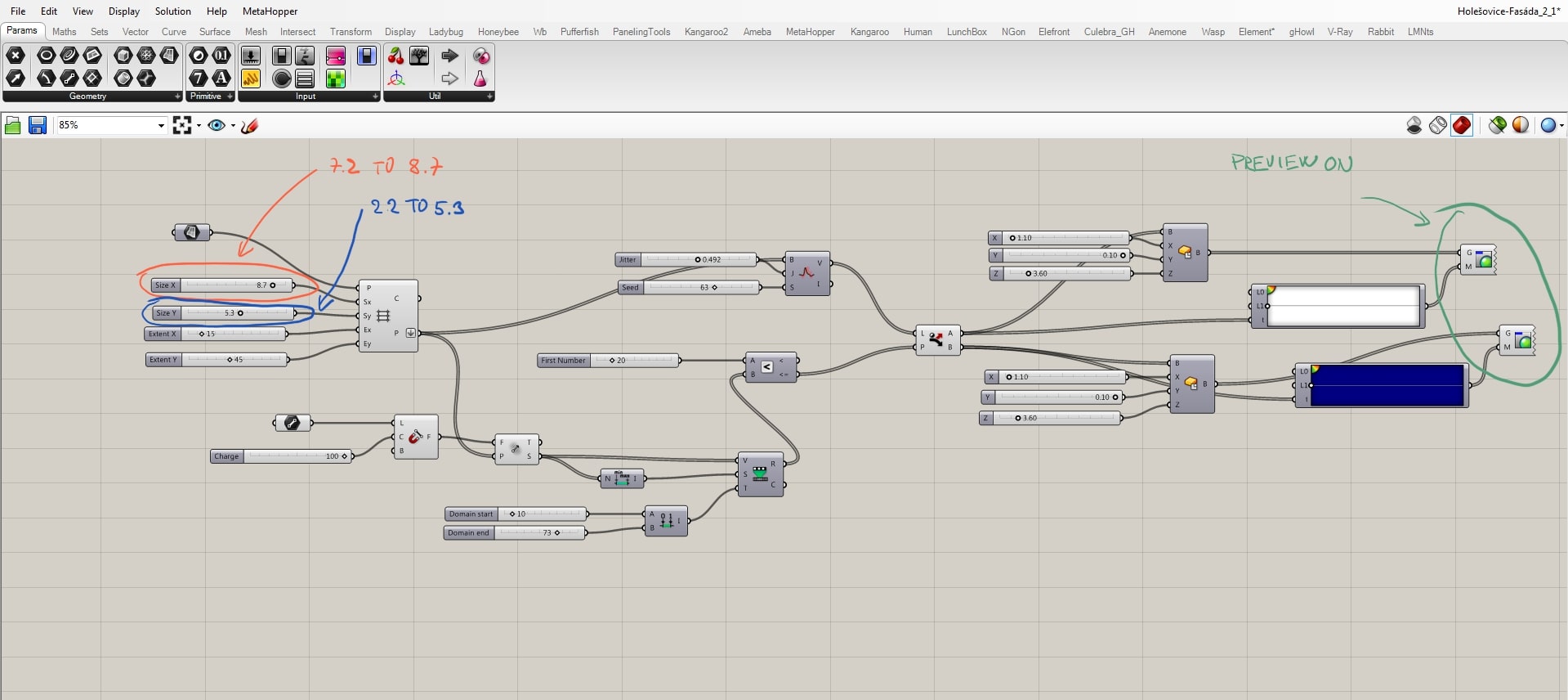
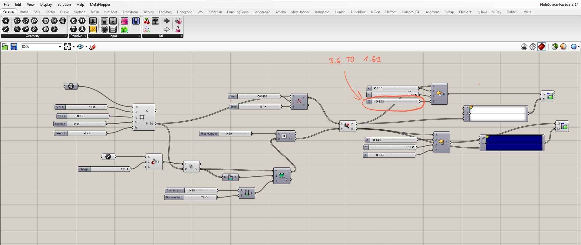
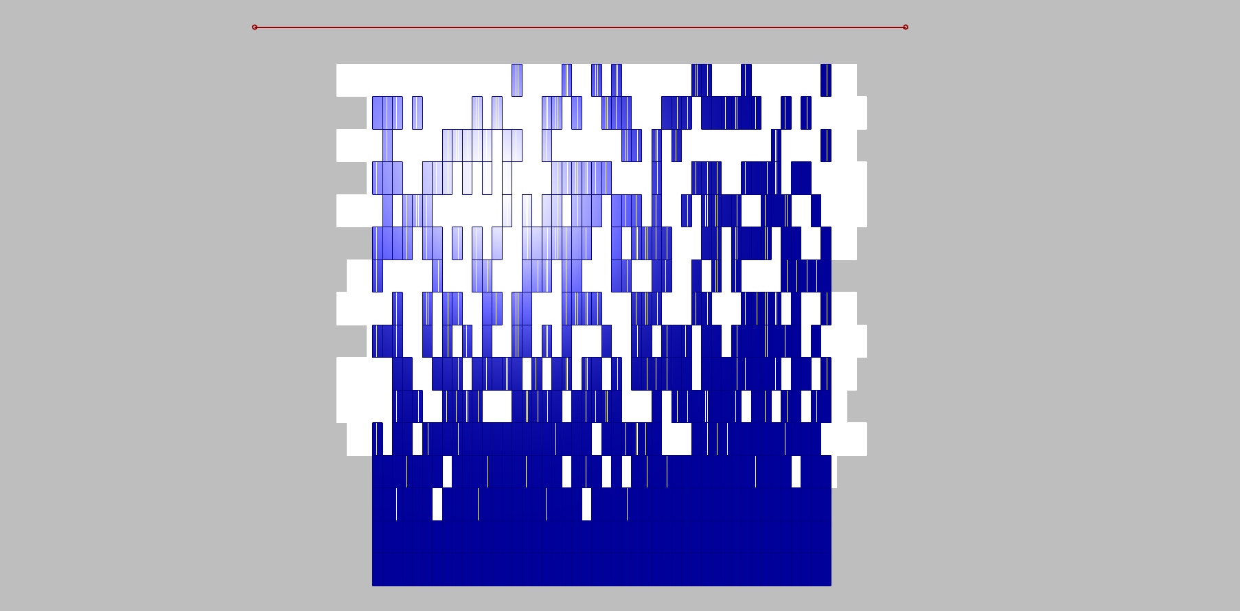
Here you can see how changes of the boxes’ measurements affect the whole project.
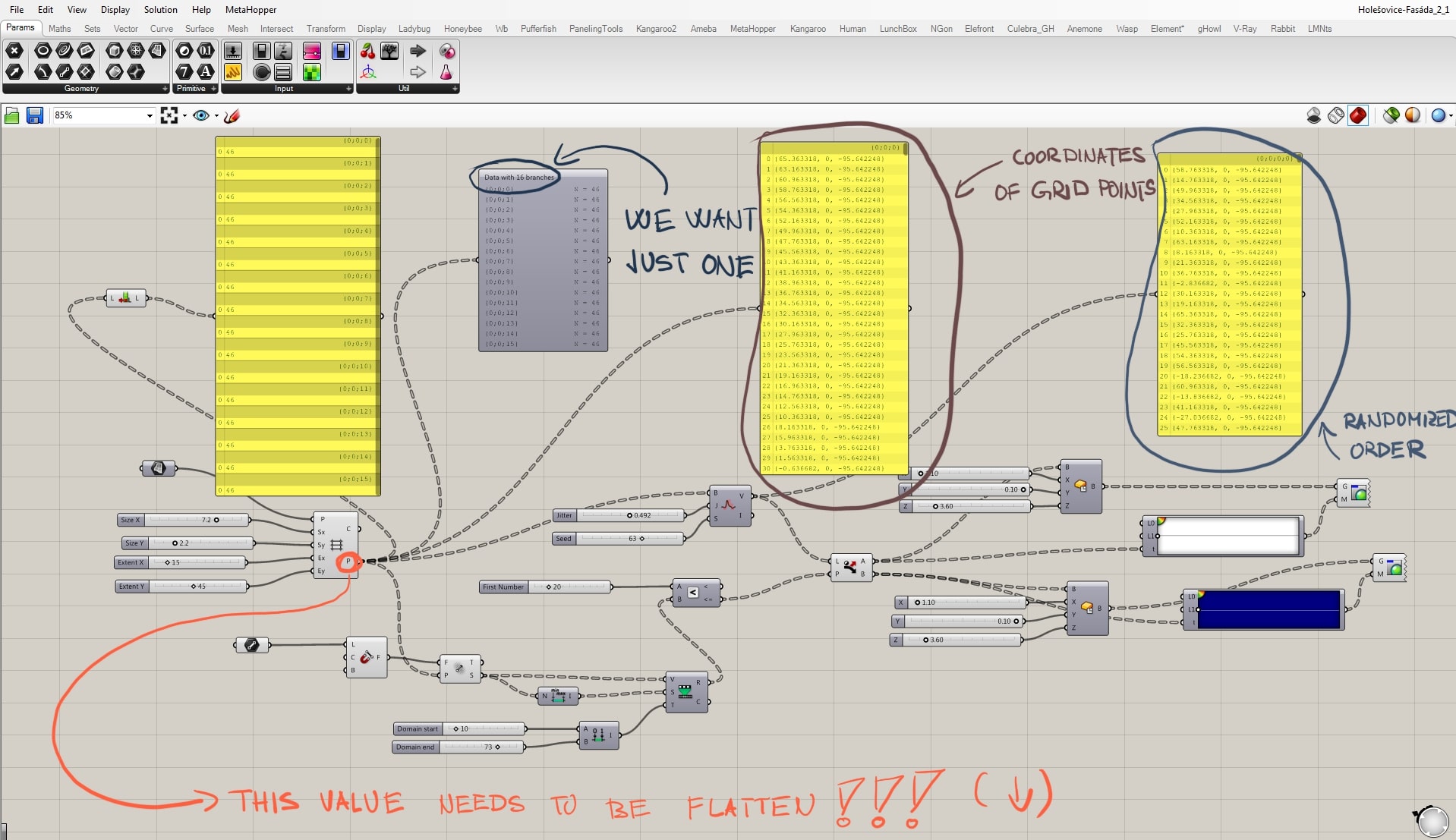
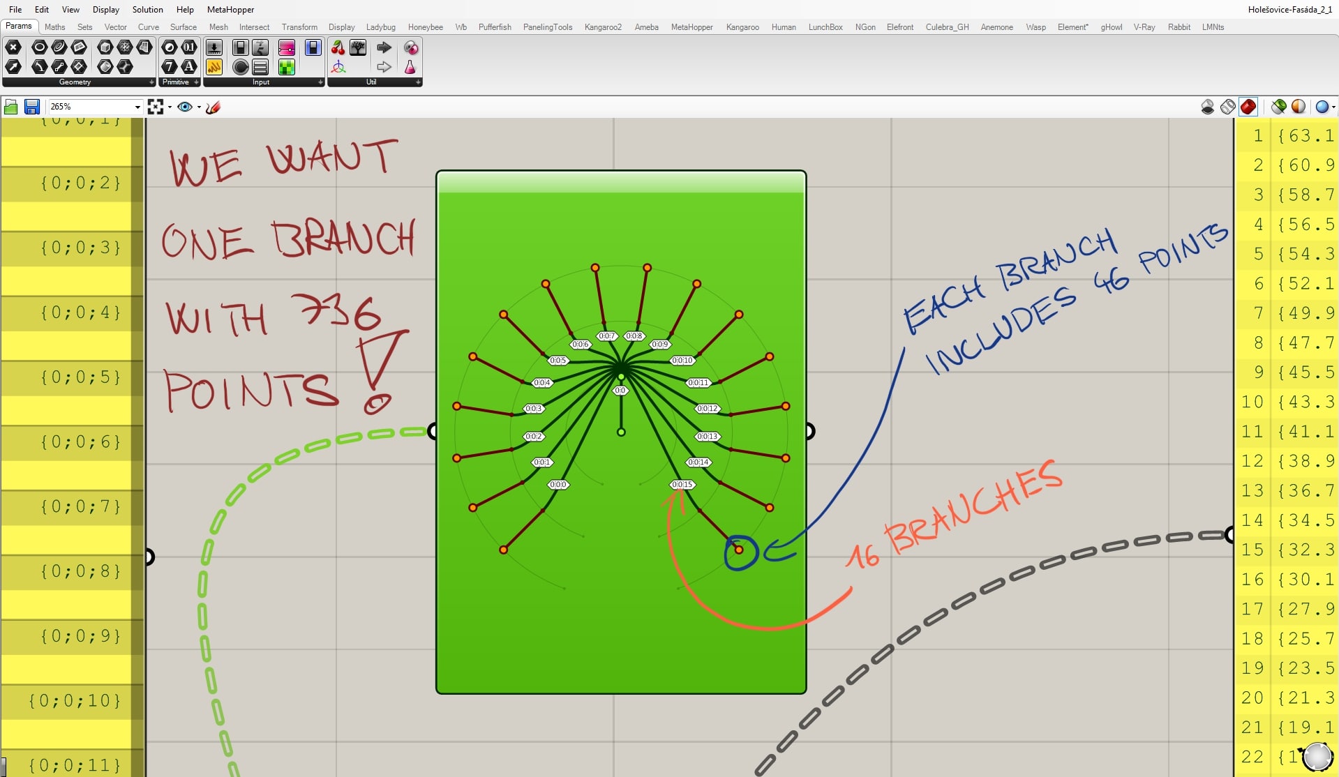
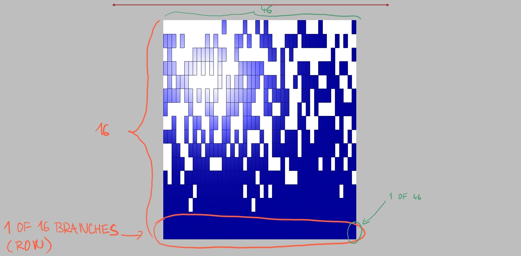
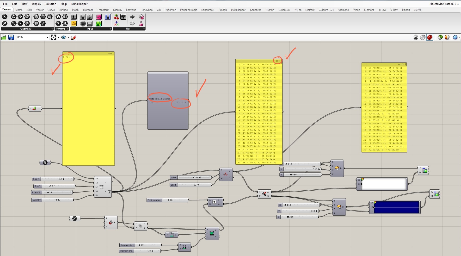
Maybe the most important thing to understand is the “data tree” mechanism. The output of the grid are coordinates x; y; z. However, without any intervention, these coordinates are being systematically sorted into separated branches with certain amount of individual items. In this case, branch is a row in the model, so we have 16 rows/branches. Each row has 46 individual boxes. This division may be useful in other types of scripts, but not in this one. Altogether we want just the boxes, its coordinates. There are 736 individual boxes that we want to put just in one branch. That’s what flatten is made for. It flattens informations into just this group/branch of individual units. Thanks to that, we can then easily randomize their positions which is what we want for the design. With the system sorted into branches, the script would not work as you can see in the picture.
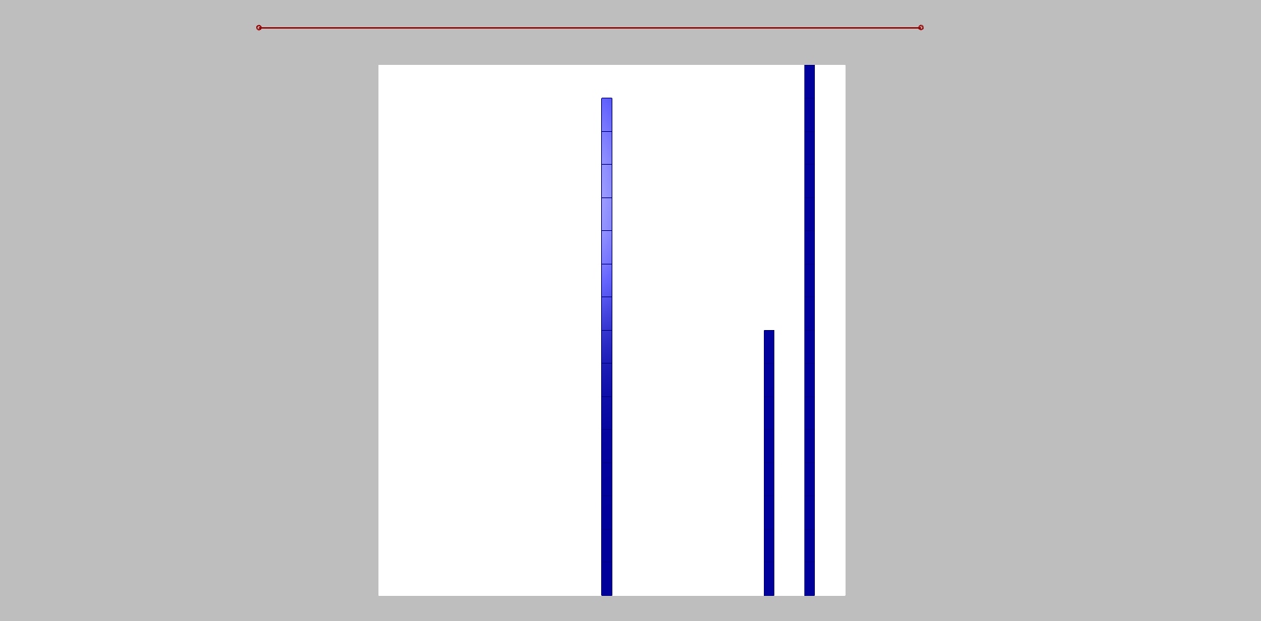
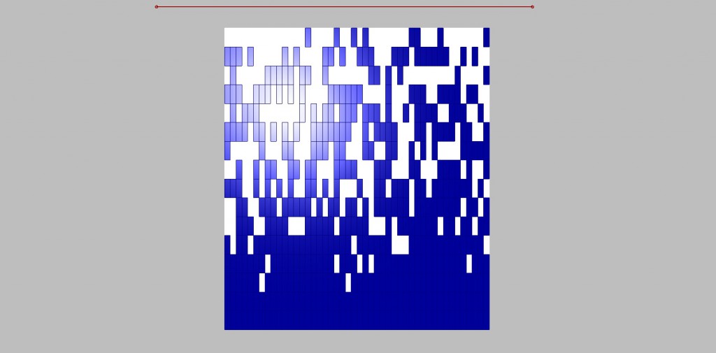
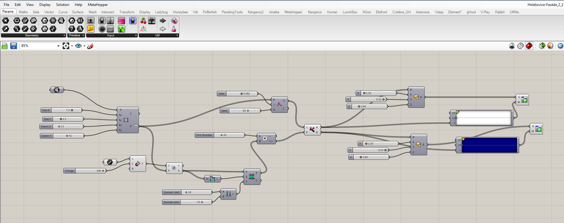
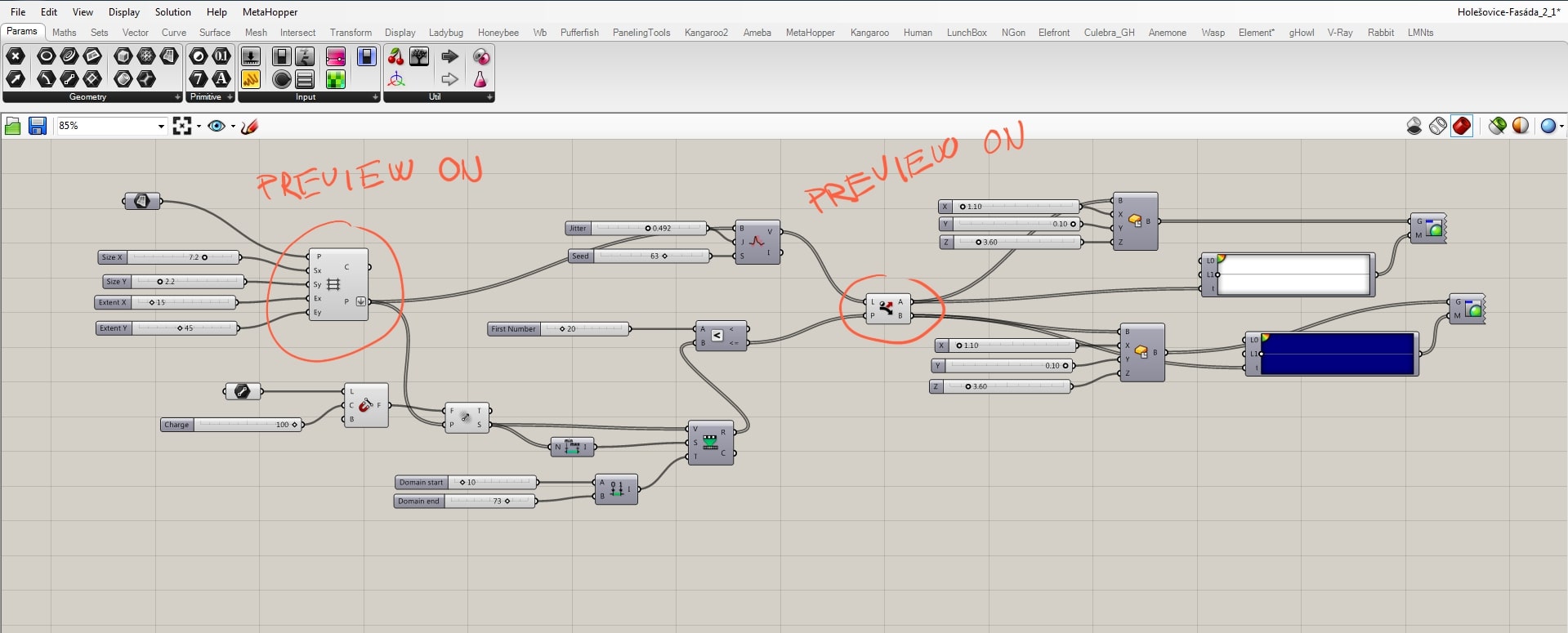
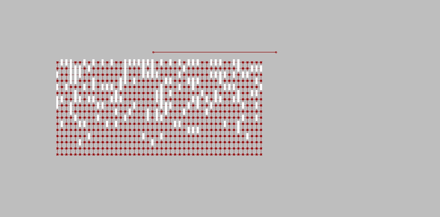
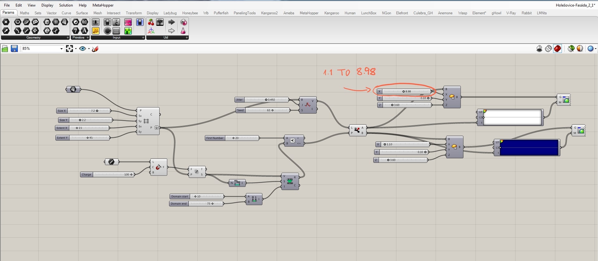
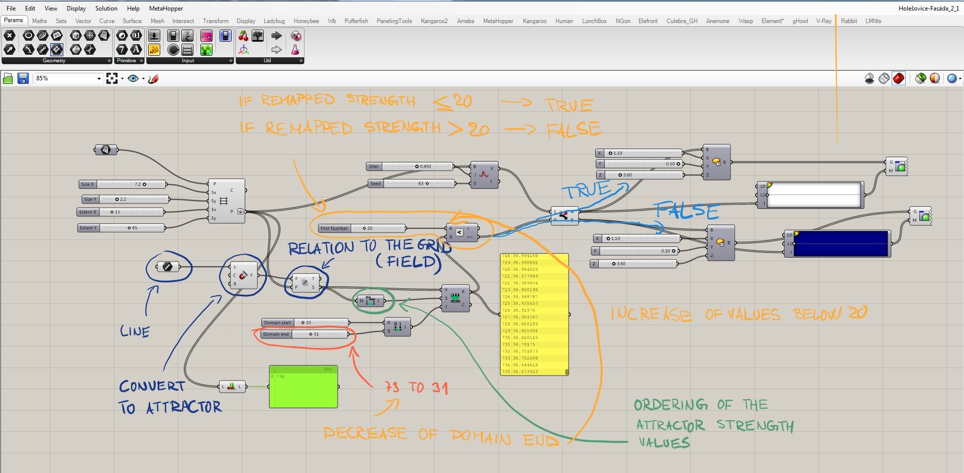
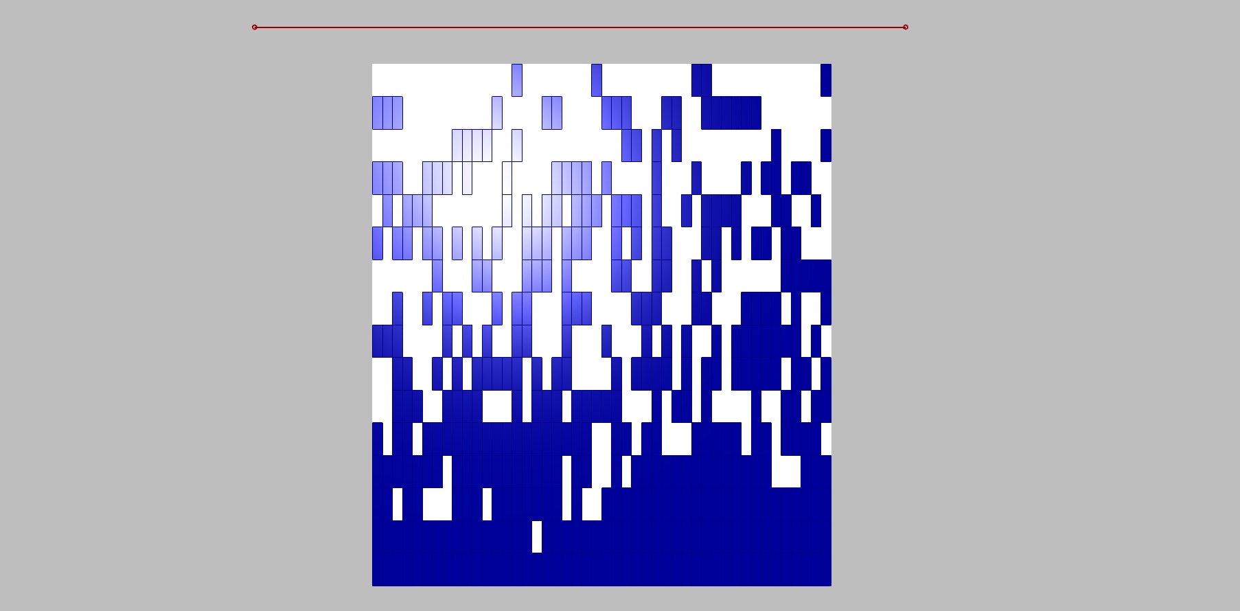
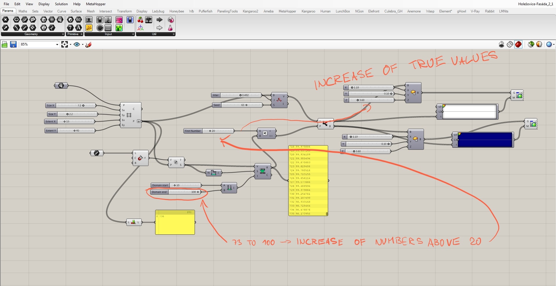
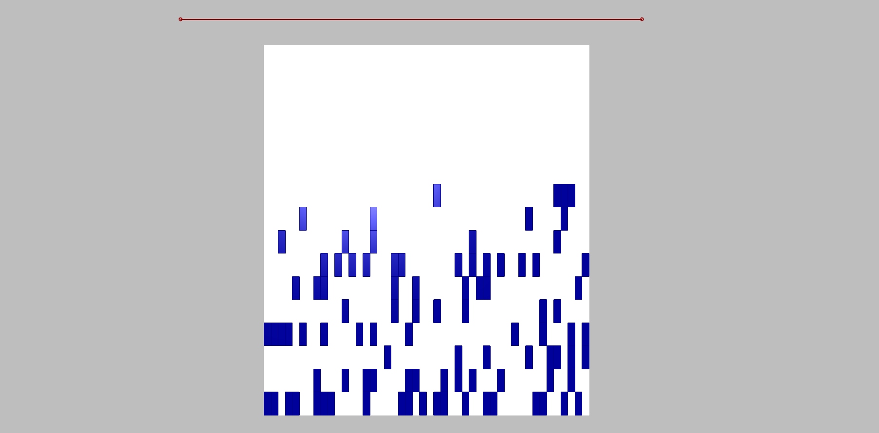
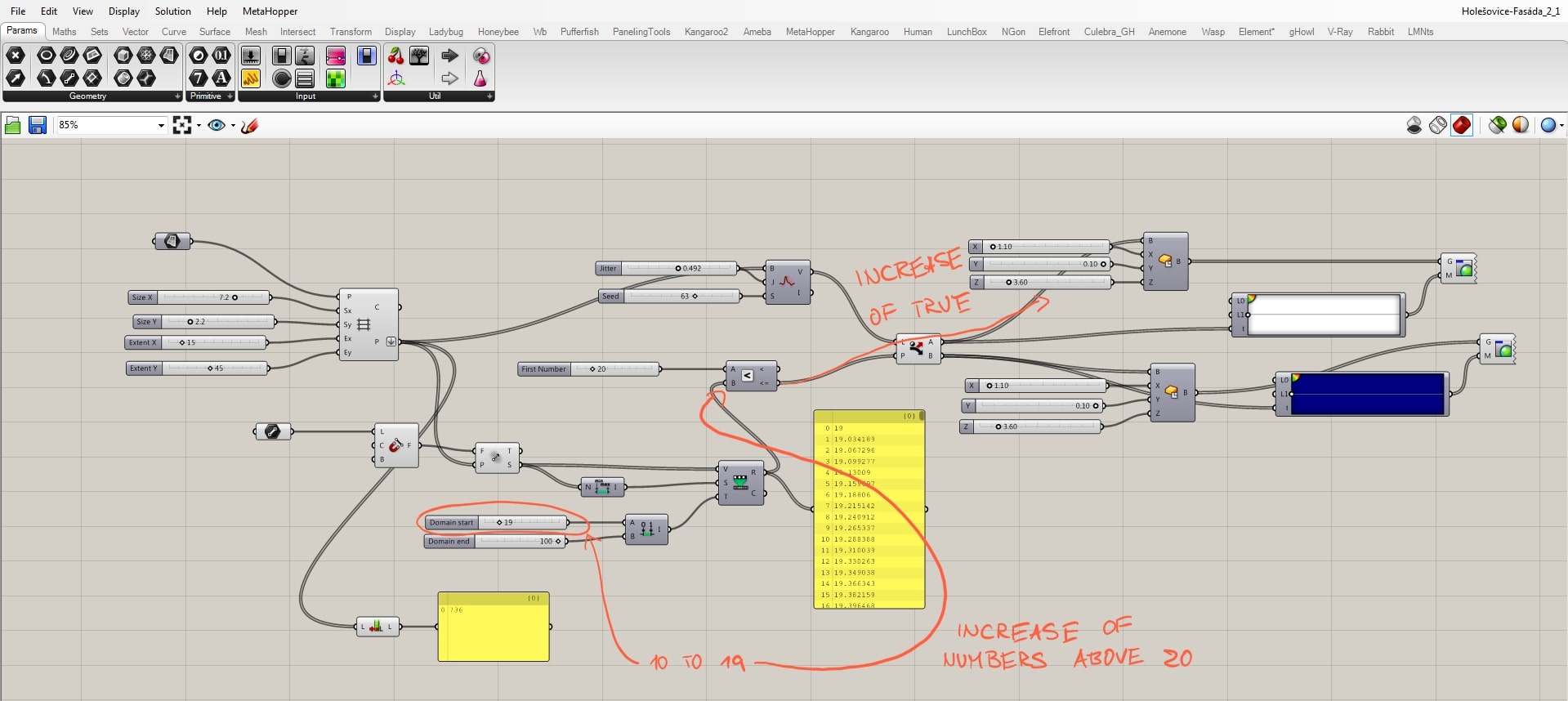
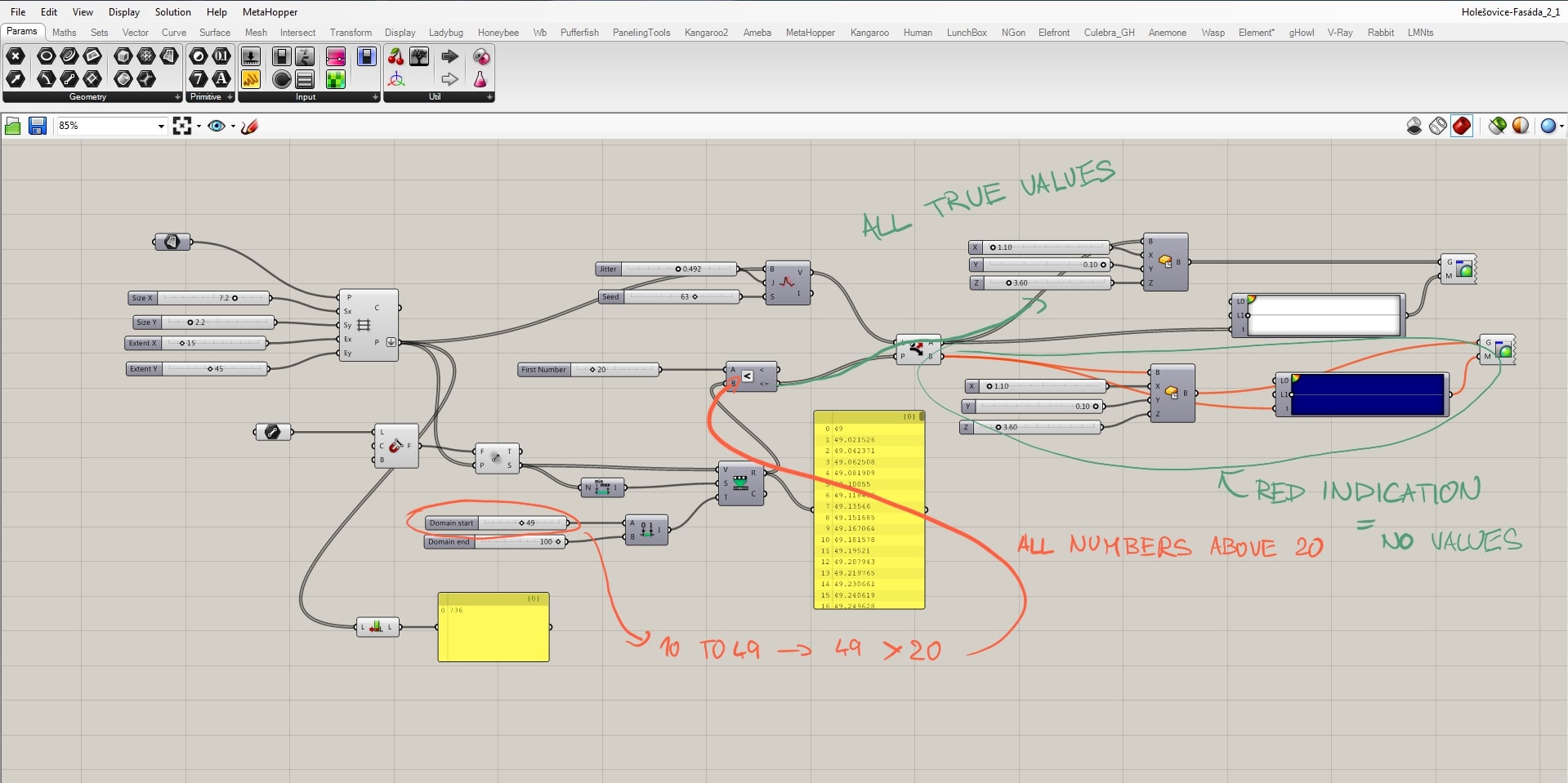
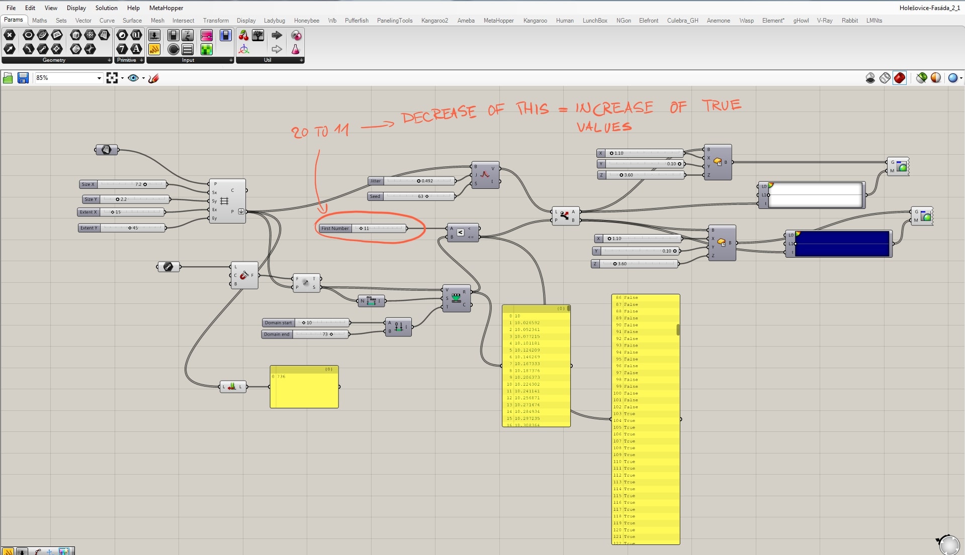
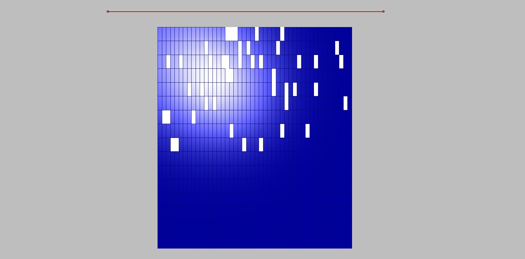
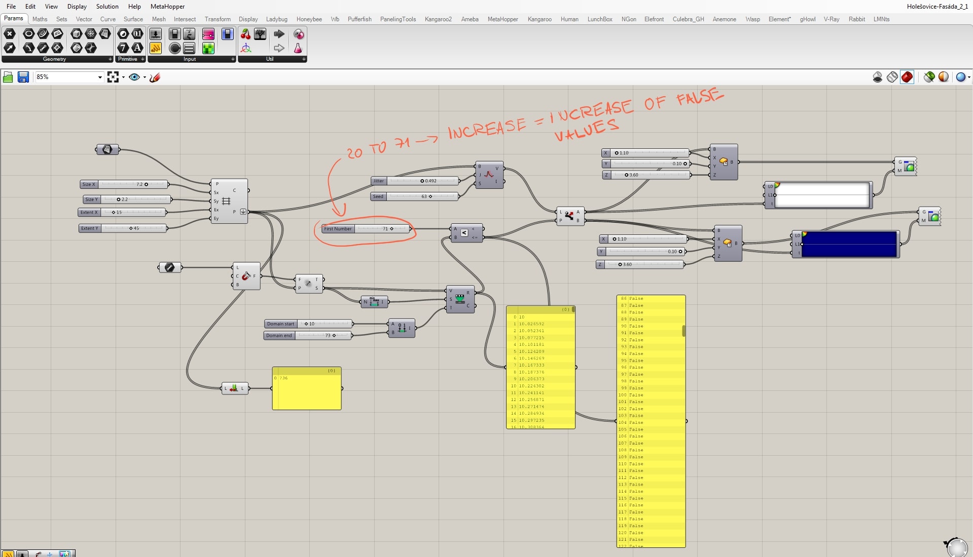
The whole concept of the script works on a principle that there is a certain relationship between the grid points and the attractor, and we want to manage it. Line creates the attractor field by evaluating the distance between grid points and the line. These “strengths” ordered from min to max by the “bounds” component are taken as the source for remapping. We need to remap these values, because only then we have control of what is the output. These remapped values are evaluated in the relation of A<B where B stands for the remapped and A for a new parameter. It is necessary to say that above certain field’s strength the boxes become blue and below it white. A<B component’s output are TRUE or FALSE values whether the relation was correct or not. Now we define that TRUE values become white and FALSE become blue by the use of the “dispatch” component.


The relation between the field and grid points is fully manageable, but we can only define the amount of white and blue boxes. We still want to randomize them, and that we can do by the “jitter” component. Jitter takes the initial order of grid points and mix them according to the jitter value. By doing this we destroy the clear relationship with the other half of the script, because that works with the initial order. For that reason, with a certain amount of jitter some white boxes supposed to stay white become blue and vice versa.
Below is visible decrease in jittering.
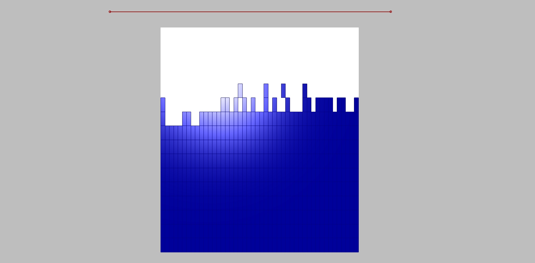
Increase in jittering

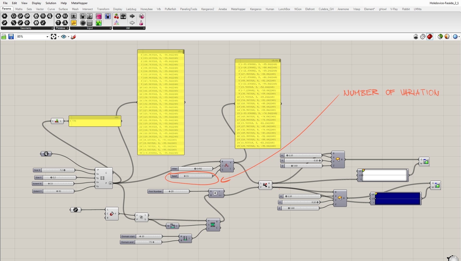
The seed value stands for the variation number, because with the same parameter setting, we can bring large number of variations according to the scale of the grid.
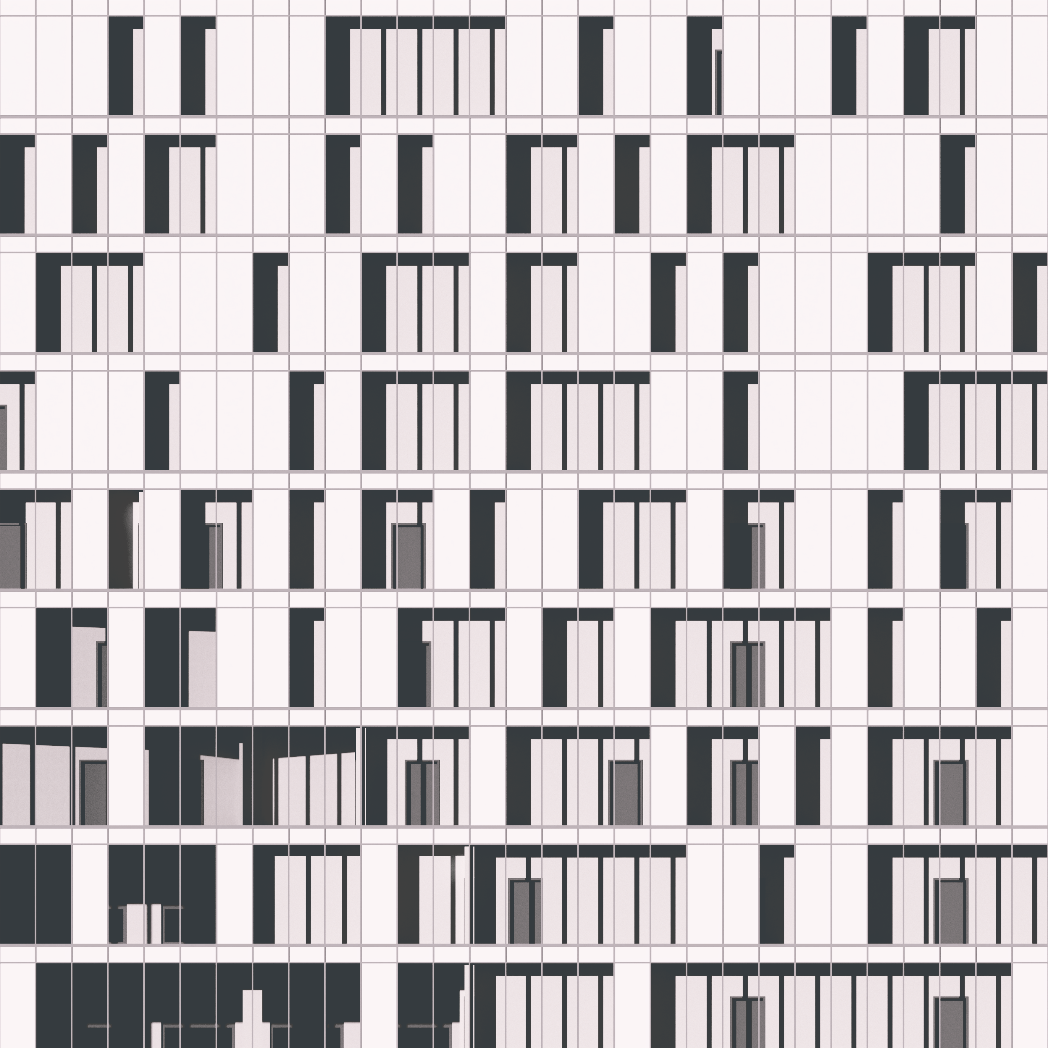
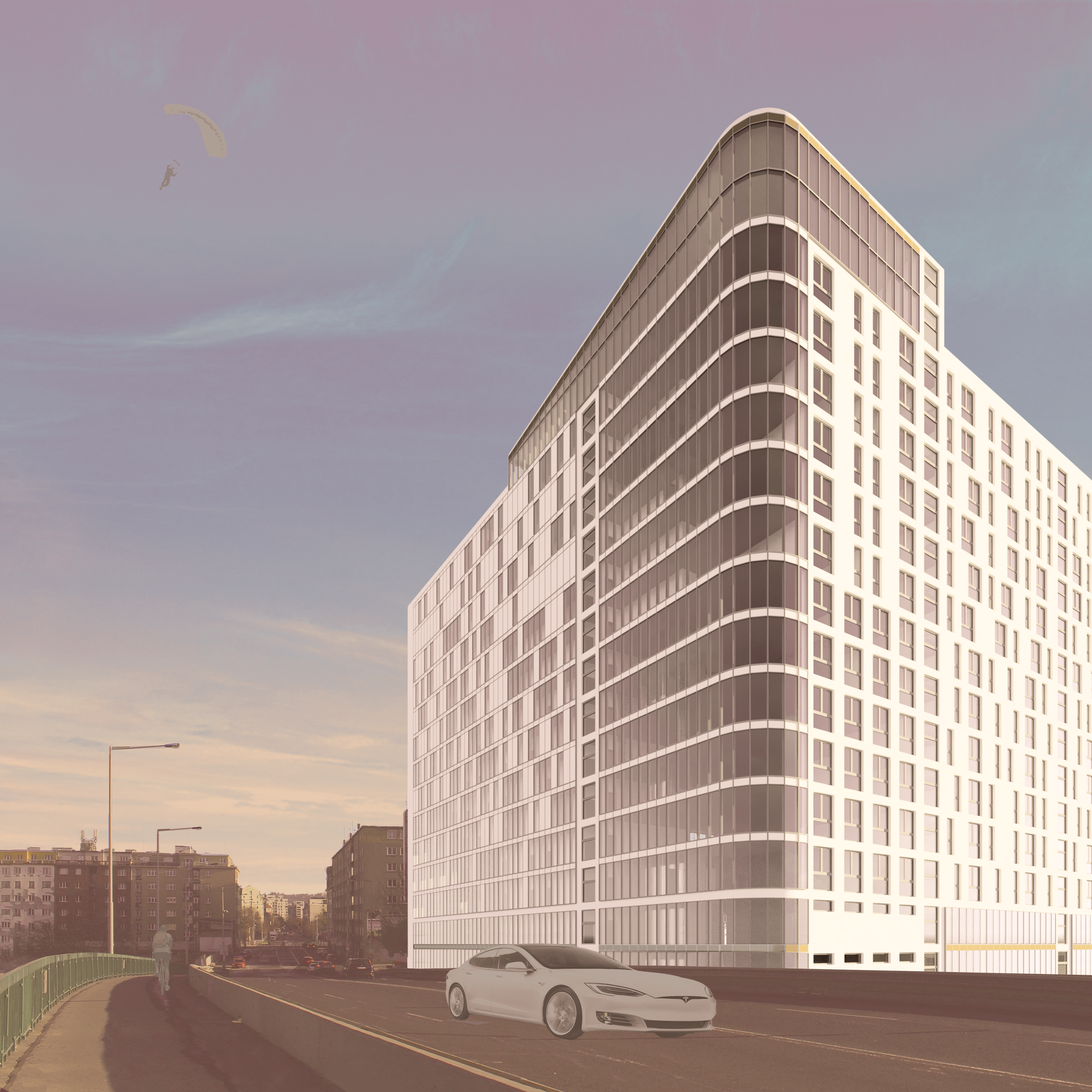
I used this script as a design foundation for a curtain wall façade in my semestral project. In the pictures below you can see the final state.