
1, Concept
Main goal of the work was to analyse visibility in streets of locality Petrská Čtvrť in Prague. The analysis was purposefully made with standing cars on streets, and then without them to show how big of an impact standing cars have on visibility in the streets.
2, Scripts
Overview of the main script:
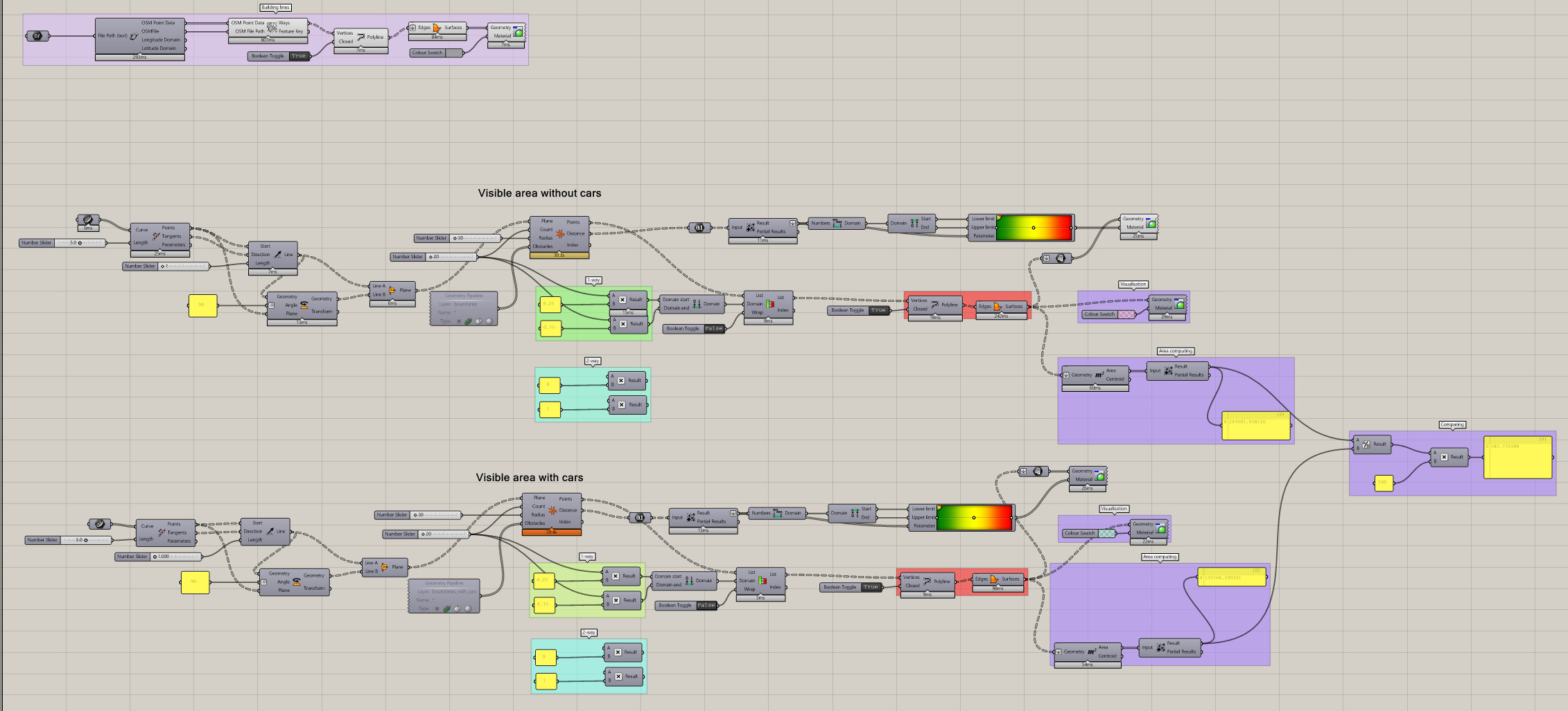
a, Data
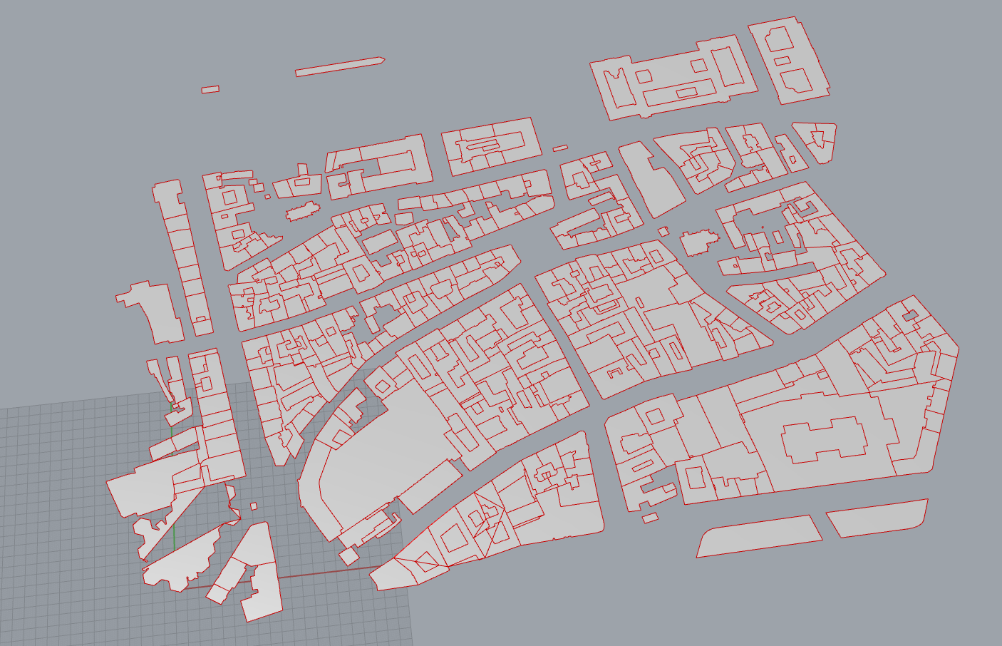
First, we have to get boundaries of buildings of the area, for that i used openstreetmap.org and downloaded the osm file of the area. With that i was able to upload the data with Elk plug-in into grasshopper.
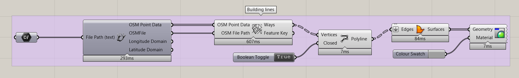
First i add “file path” locating the file, add “location” and “OSM data” from Elk plug-in and make polylines out of it and fill the insides.
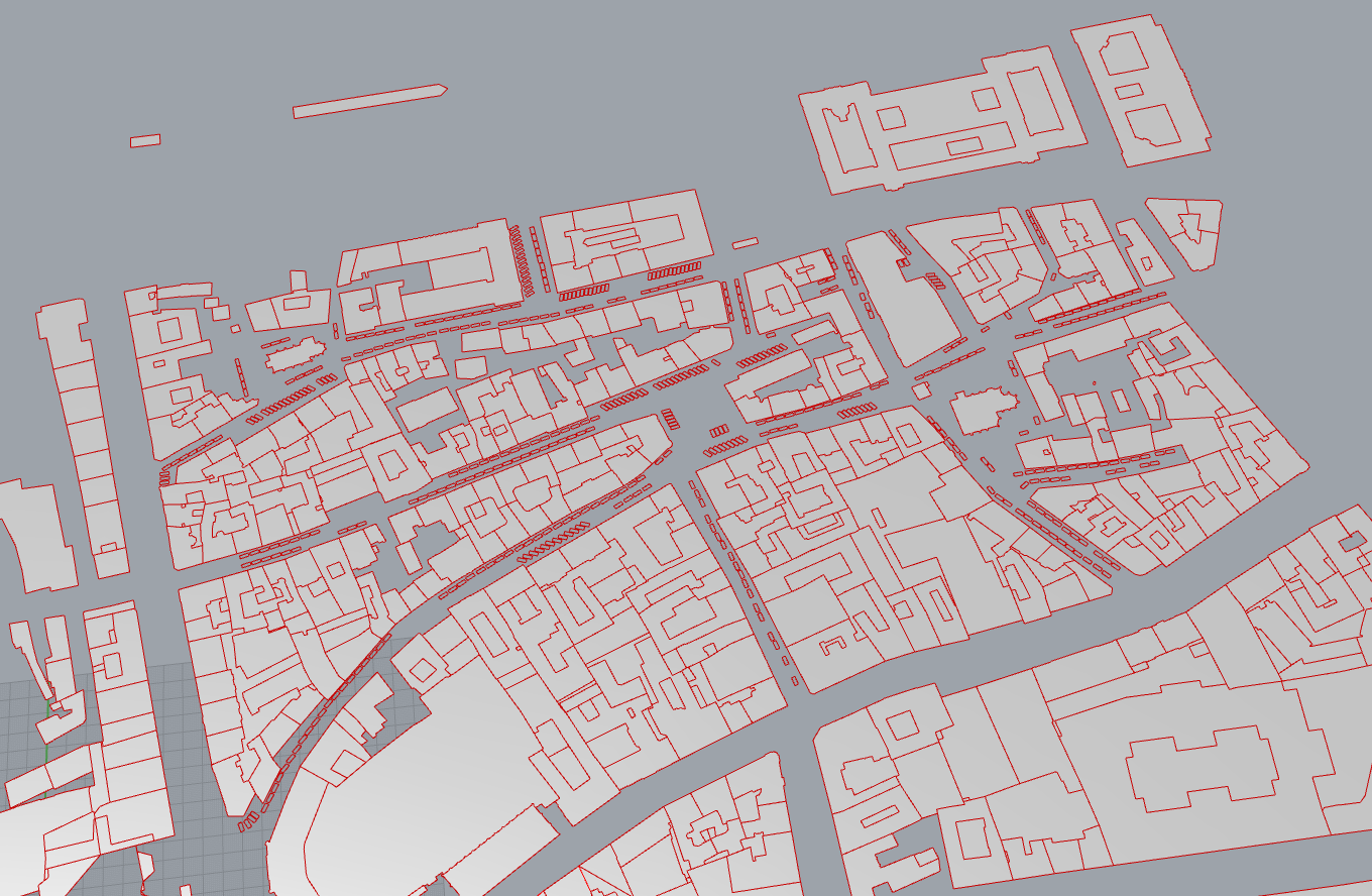
As for the cars, i didnt find any online file for the parking spots, so i had to make them the old way, handly draw each one. The cars and the buildings have to be in the same layer in Rhino. For the comparison later on, second layer has only buildings.
B, Analysis
With the data being done, we can now decide what kind of analysis it should be. I wanted to make path across the locality to analyse all of its roads. So i drew polylines through the streets and uploaded them to grasshopper.
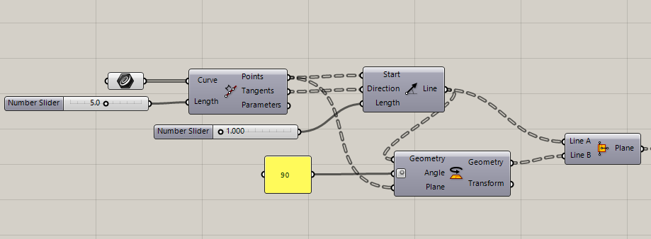
Then i divided the polylines to same length to make observation points for the analysis and made plane in each one to prepare it for next phase.
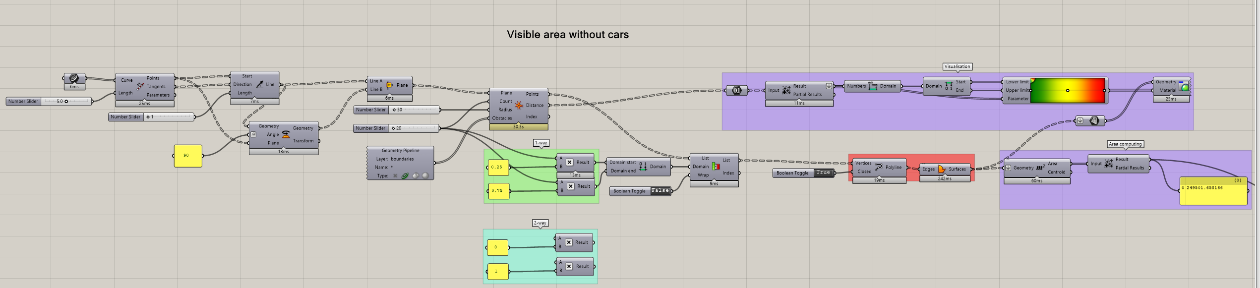
Those planes and few parameters go into IsoVist component. Now we can also upload the layer with buildings and cars. Since i want only one-way analysis (180° view from each point), ill just work with 0,5 of the count.
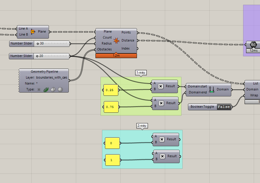
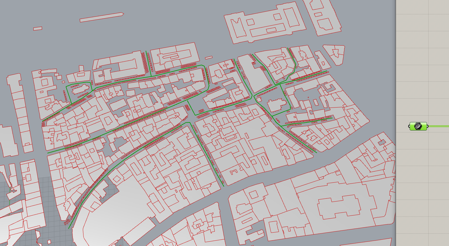
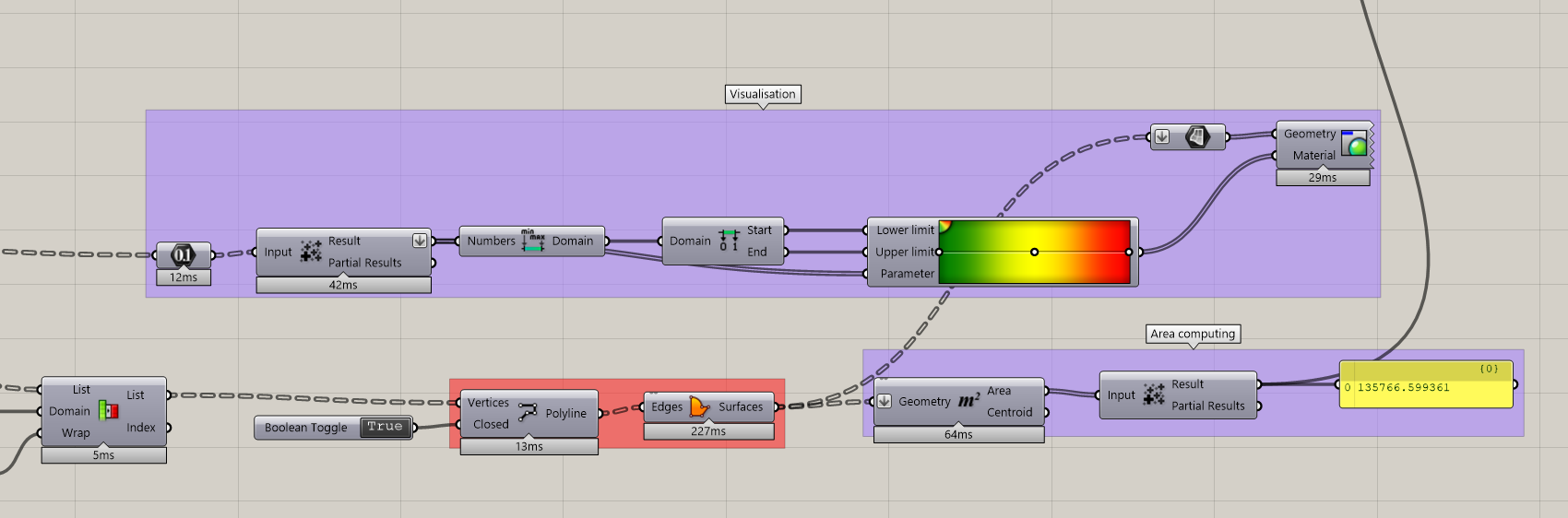
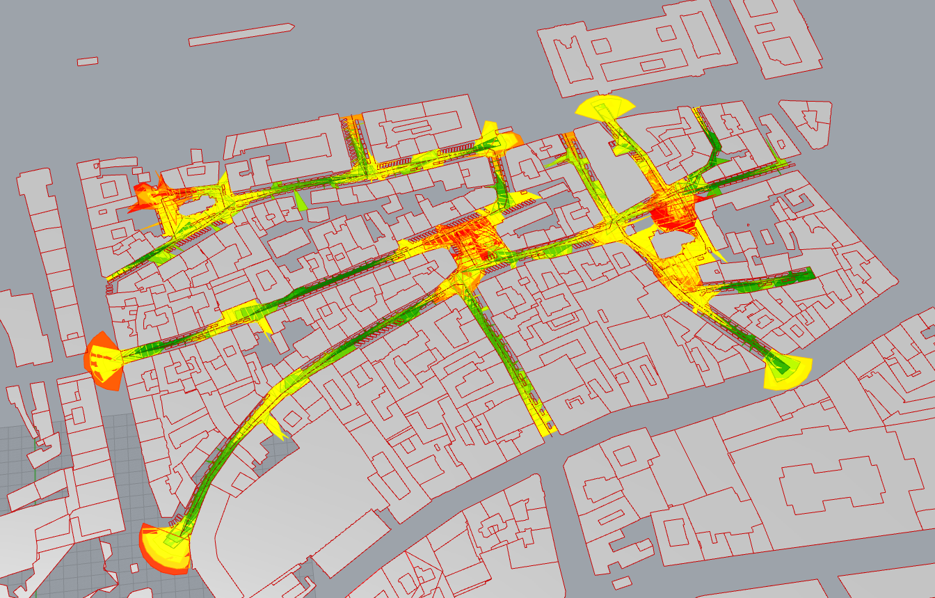
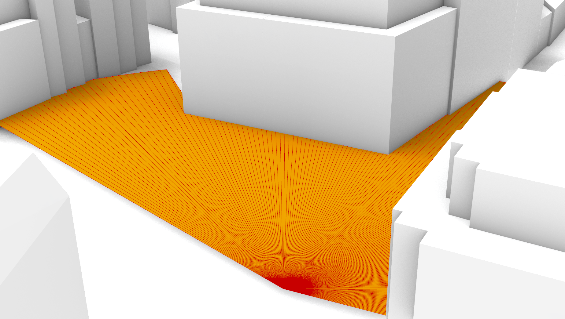
From IsoVist i use 2 outputs. Distance for visualisation and points for making the polygons. From these polygons i can calculate the total visible area of the locality. Higher lenghts of visibility are shown as red, lower lenghts as green.
Now i did the same thing again, but now without the cars. For that i will need another layer with boundaries of the buildings.
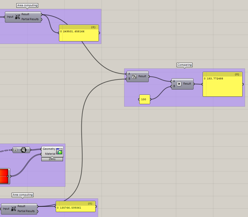
In the last part i just compare the two result, in this case the visible area without cars is 184% of the area with cars (or 1,84 times larger).
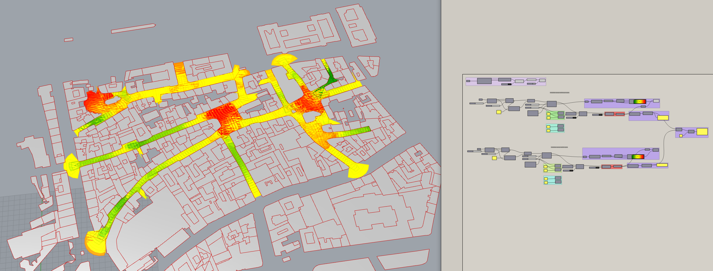
Final result, again with red being high visibility and green being low visibility:
B.2 Other types of script
With the help from decodingspaces tutorial (https://toolbox.decodingspaces.net/tutorial-2d-and-3d-isovists-for-visibility-analysis/) i was able to make another 2 scripts that can show the data in different ways.
- Point based visualisation
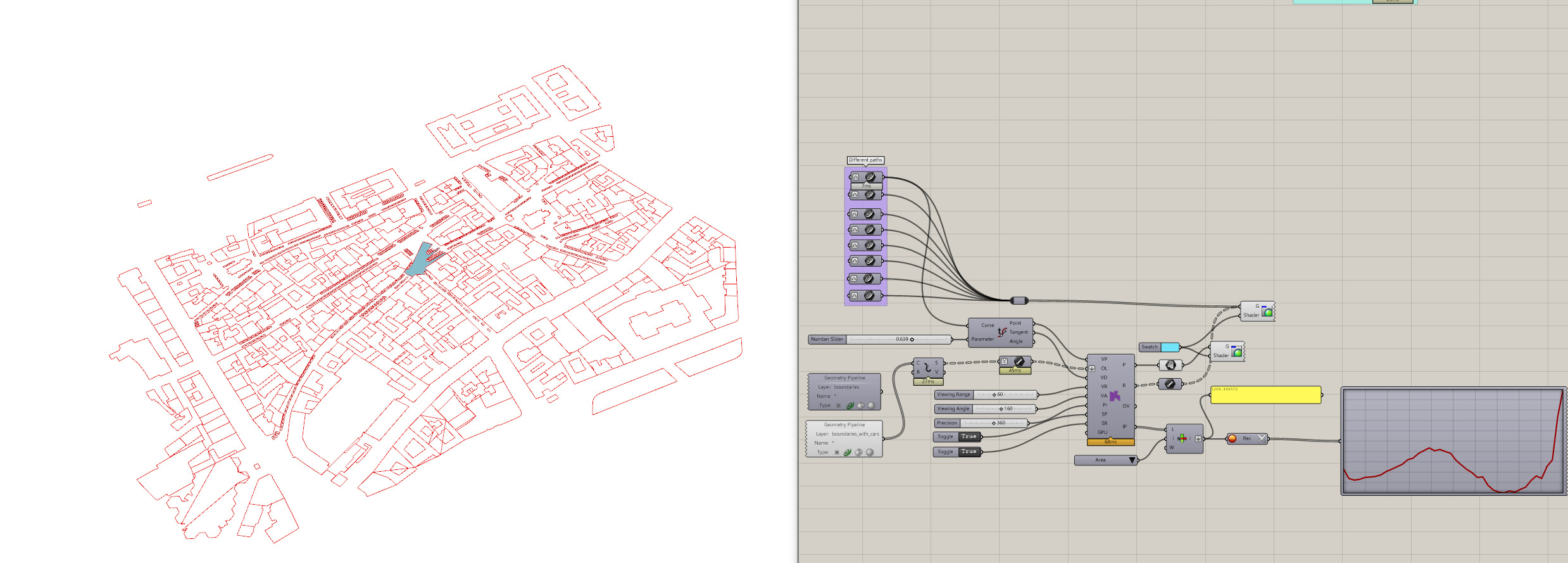
First of those two is point based visualisation along the given paths. In this script, we can connect paths we created before and upload them one by one into the GH. With “Evaluate curve” we can move along every path.
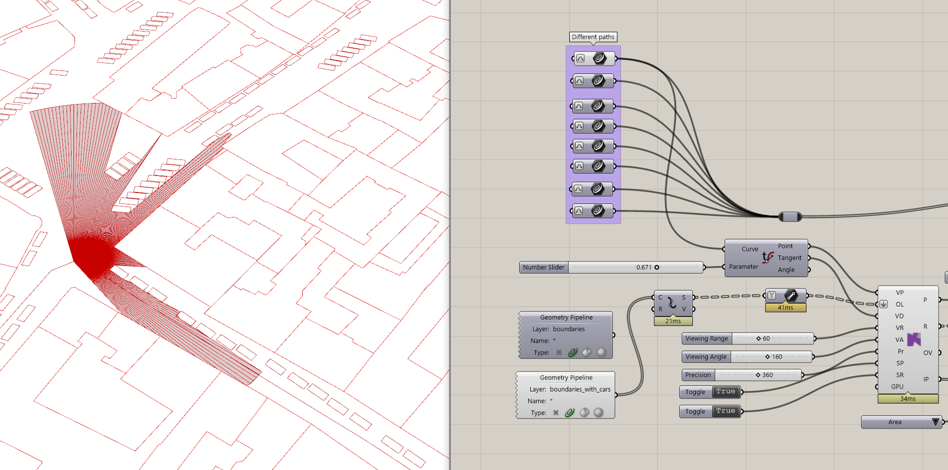
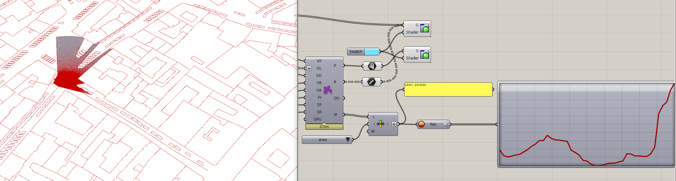
This time, we use IsoVist from DecodingSpaces plug-in. After deciding on parameters like viewing range and angle, the components gives us, among other things, area in each point on the path. We can then record those areas and put them in a graph. This script can be good for showing changes of visibility along a given path separately.
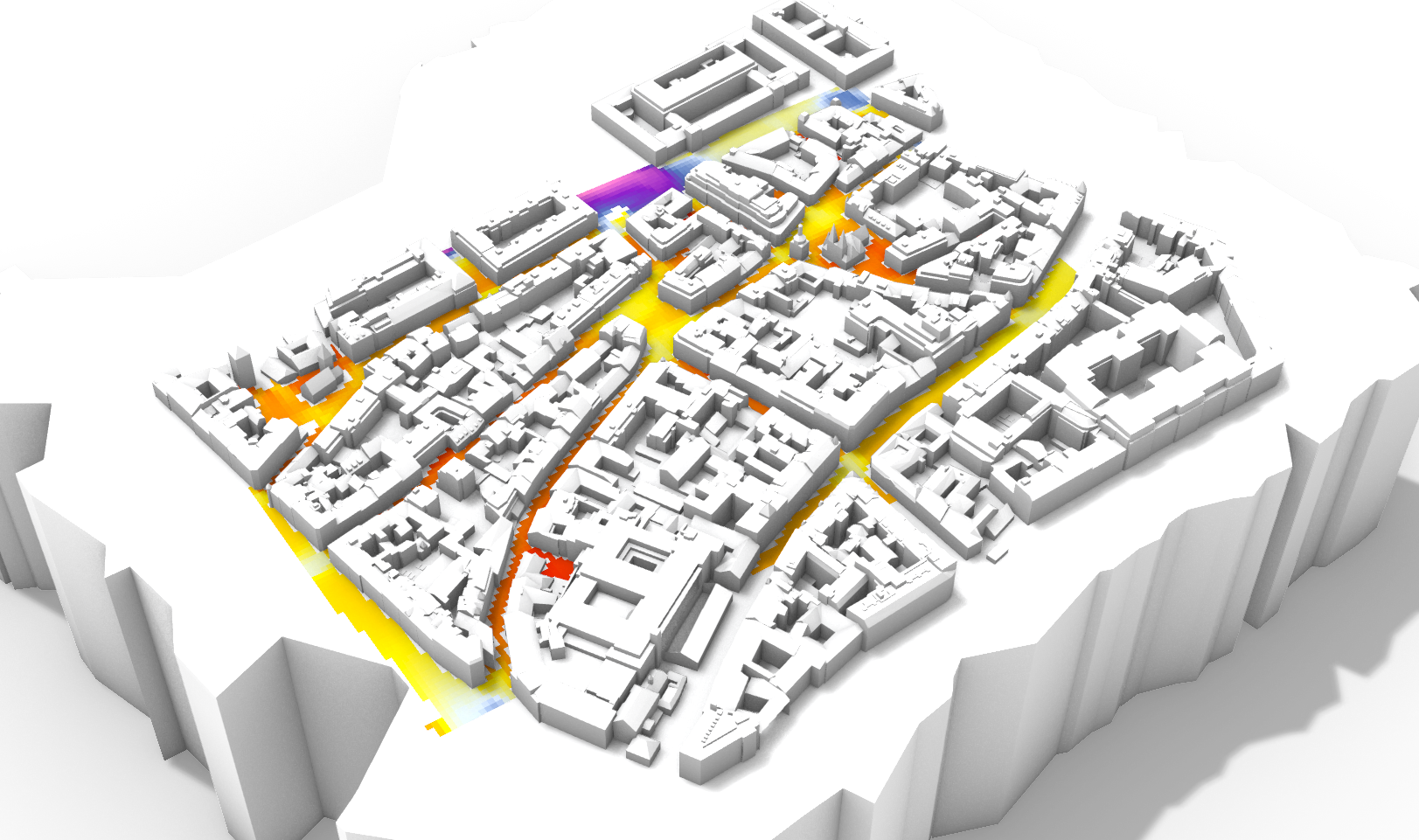
- Analyse grid
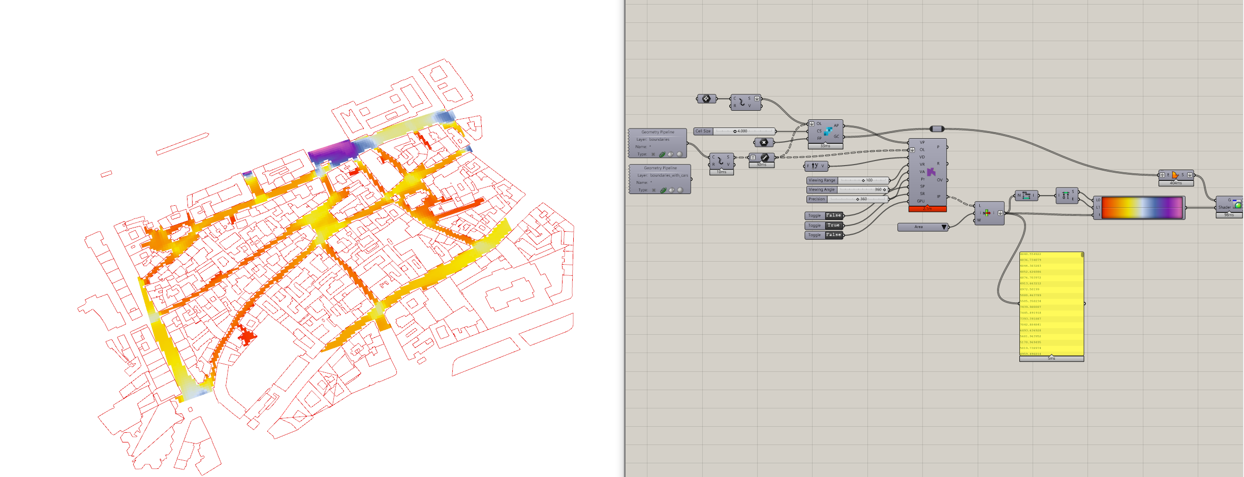
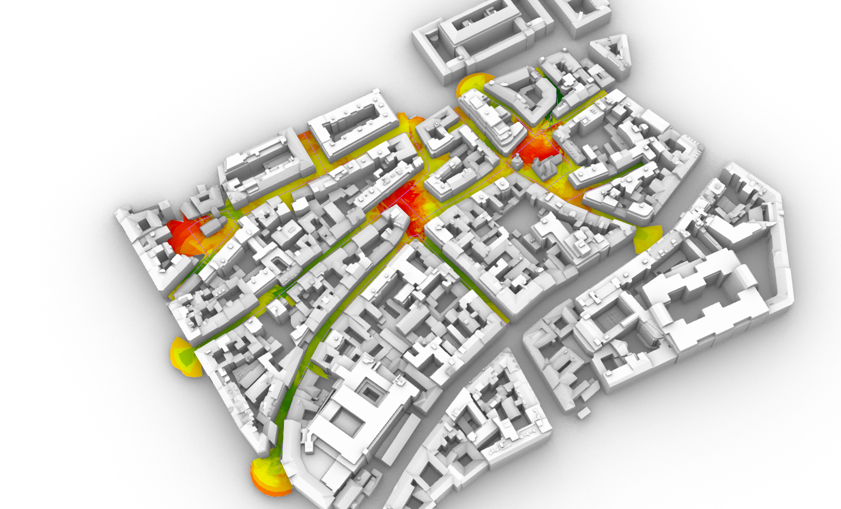
Second script is used to make a visual grid on the given area. This grid can visualise many things (like circularity or compactness), in this case i was interested in “Area”. That means the script calculates how much visible area is there from each grid cell, and then paints this cell accordingly. At the end it gives us a kind of a heat map of visibility in a given area.
First, we choose our desired grid boundary and connect it, along with boundaries of buildings, into the DecodingSpaces component “Analysis grid”. We can later connect this into the IsoVist component with stuff like viewing range and angle like before.
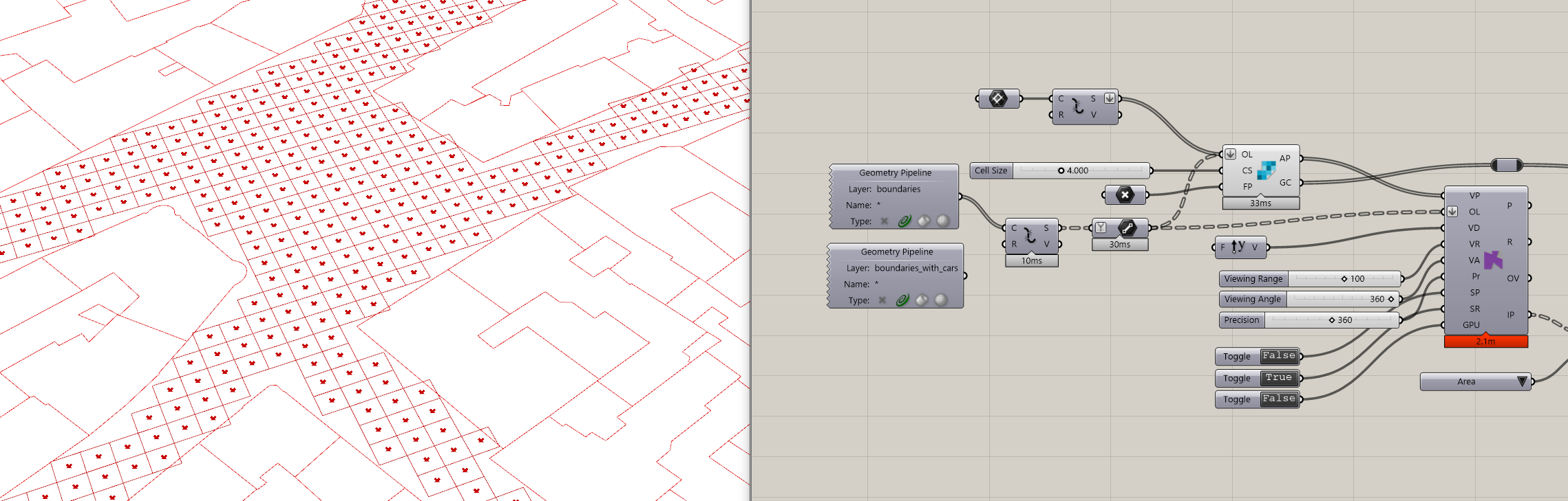
With the Isovist Properties we can get data to visualisate the grid. Here i go through the data available (click on image below to see gif). Note: With large boundary and small grid cell size, this can be pretty hardware heavy.
Images with 3D model in place:
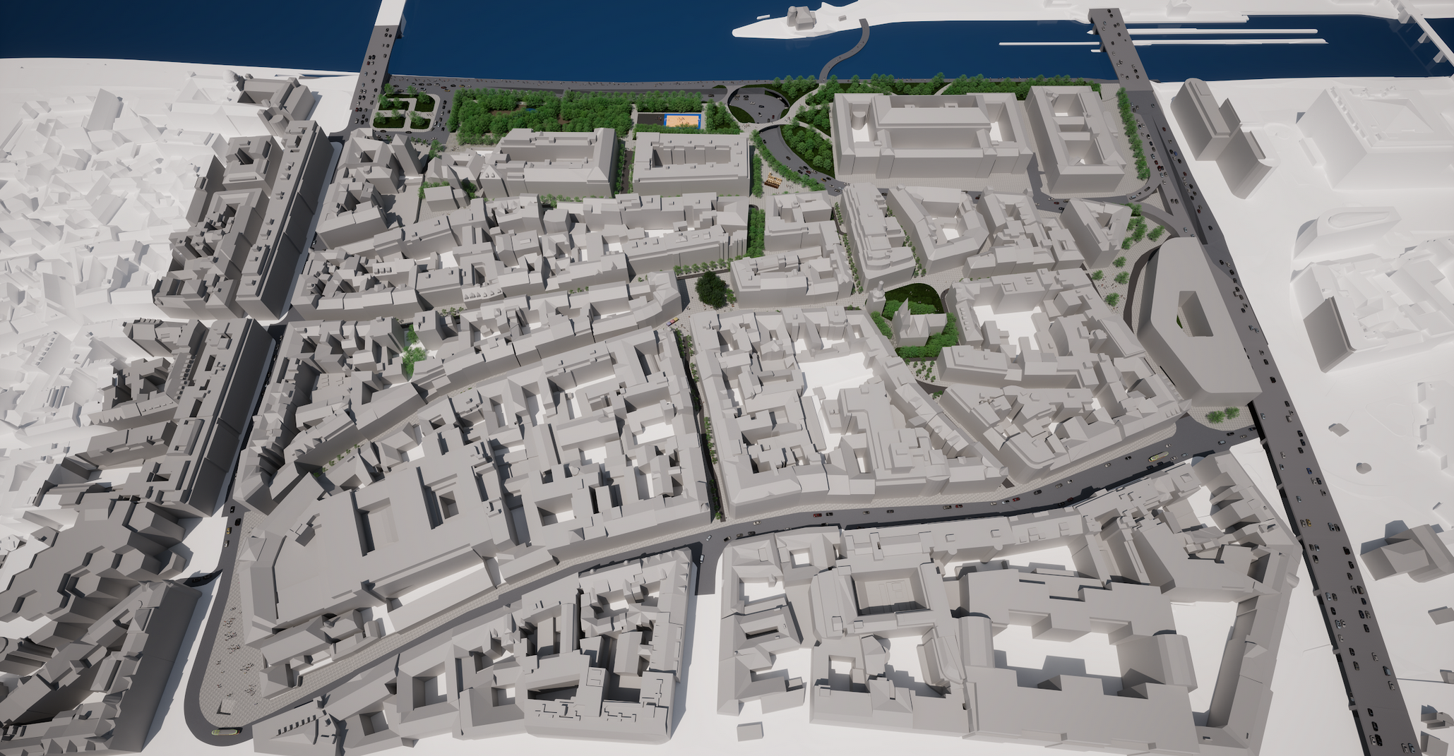
3, Renders of the area without cars
As removing cars from the locality was also my studio work, renders are also done. (Shout-out to my 3 colleagues i did the work with).


4, Thanks and files
Thanks belong to teacher for helping me with the project. Next to openstreetmap and Elk plugin authors for providing the necessary data and plug-in. Big thanks to DecodingSpaces for their amazing work, plug-in, tutorials and example files i could experiment with. Lastly to other online tutorial’s authors from which i was able to learn.
Under are files to download (terrain isnt included in Rhino file due to large file size).