Landbridge

Aim

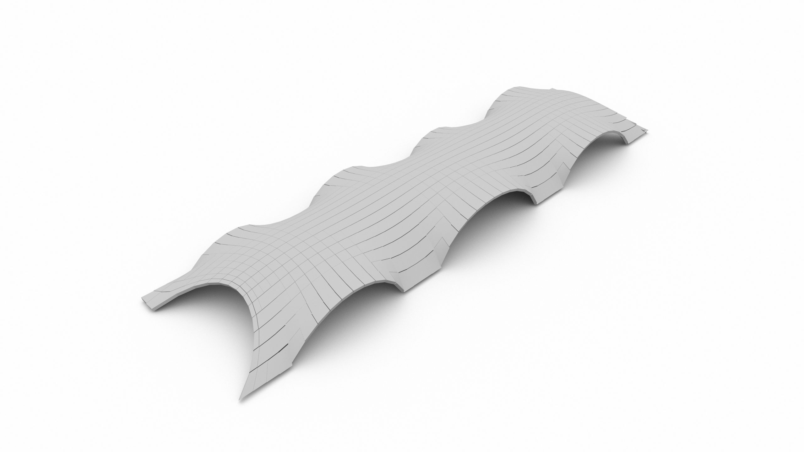
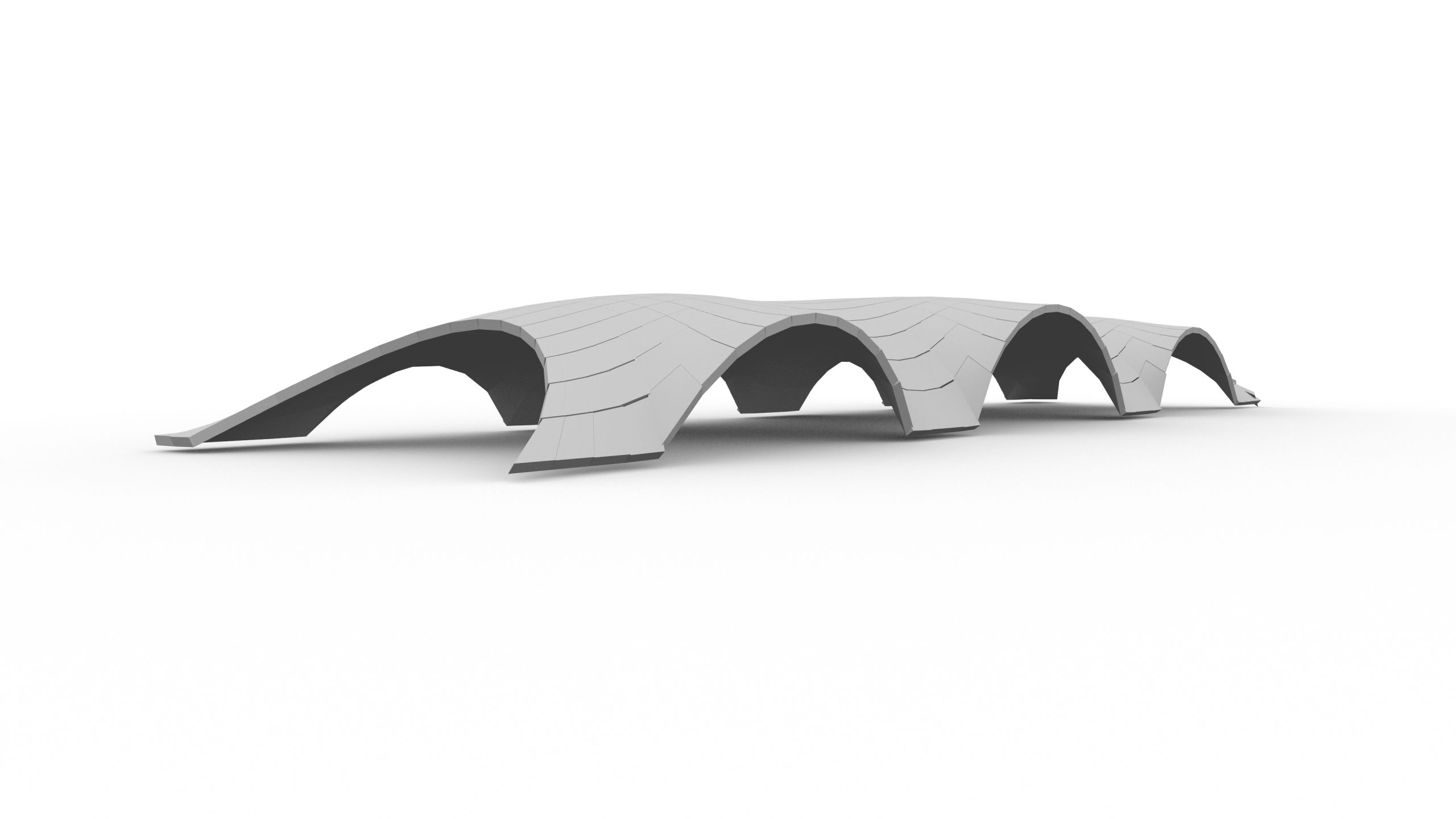
The exercise aimed to create a script using the Kangaroo plugin to design a land bridge over an existing railway track. This script can be used as a form-finding exercise with parametric variables. For my studio project, I have two parcels of land cut through by a railway track. So, this land bridge was conceived as a solution that acts both as a tunnel for the train and as an extension of the landscape to connect the two parcels into a cohesive landscape park.

Step 1

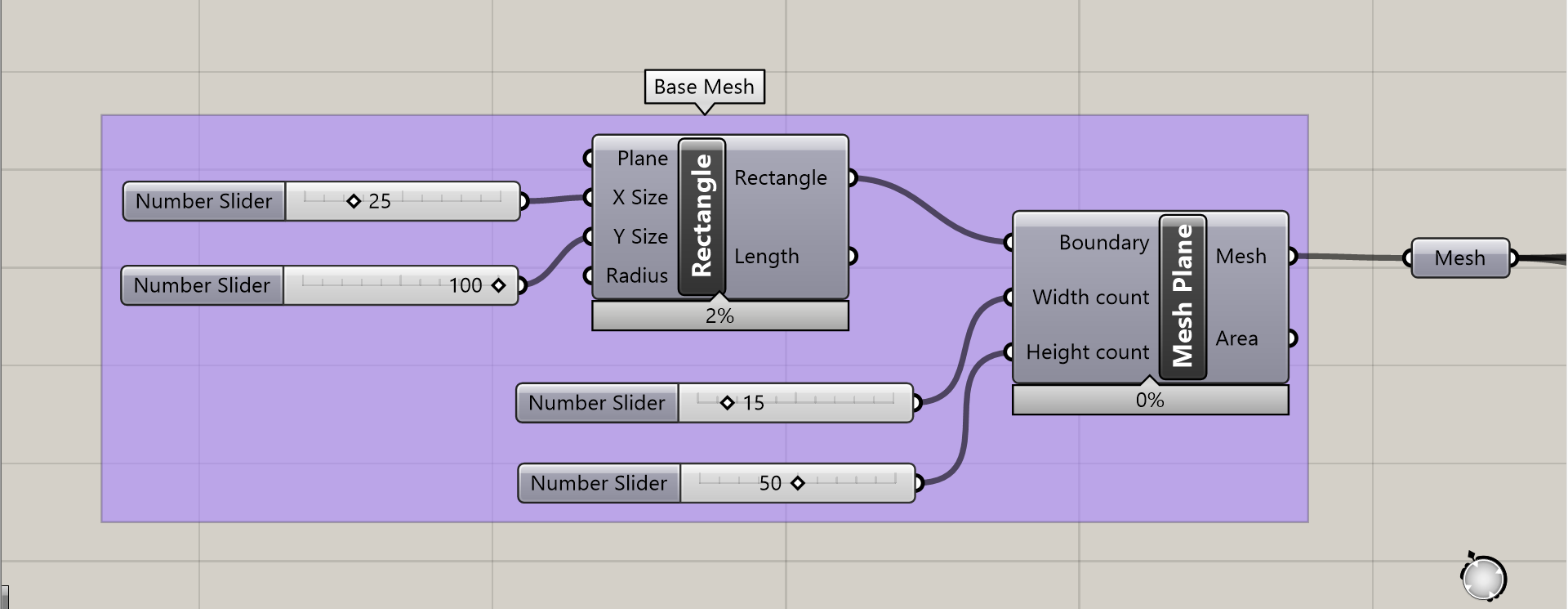
1. I started with creating a basic shape and giving it the dimensions of 25X100 m, which would act as a framework for the base mesh.
2. Then, I made a mesh plane out of it, which would be the subdivision of the plane.

Step 2

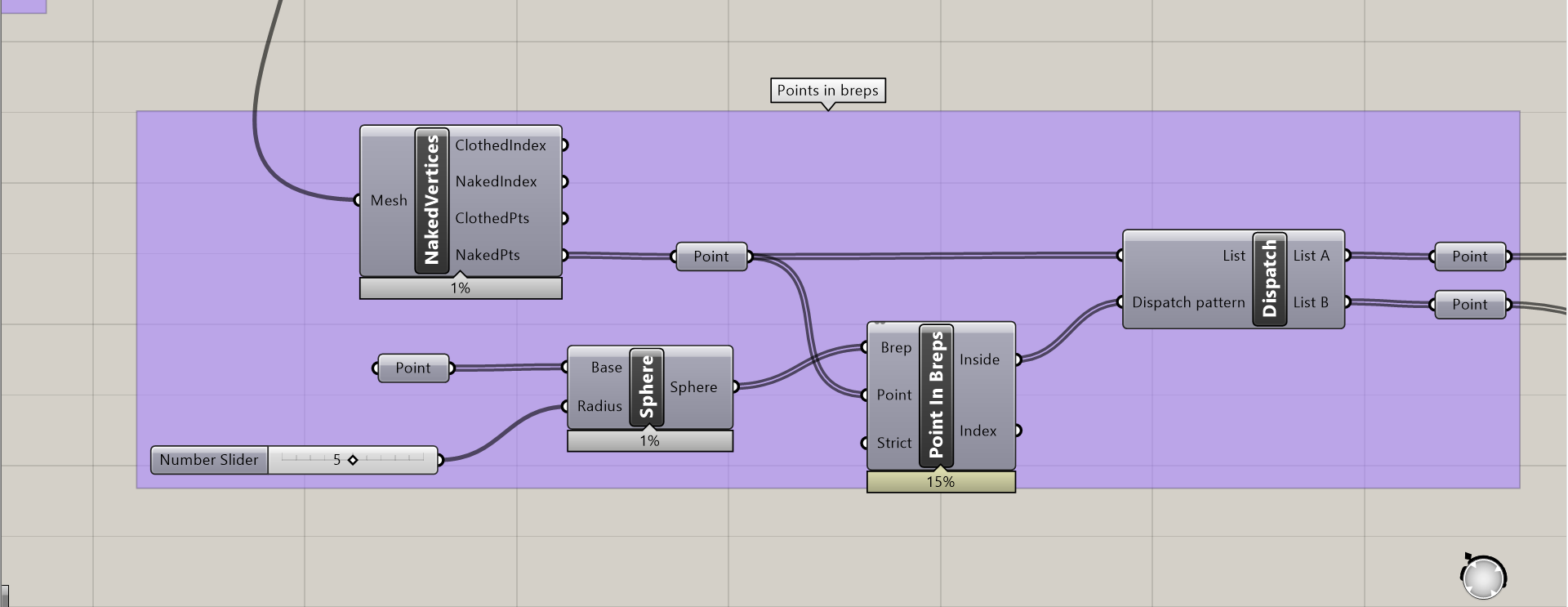
1. I used the “naked vertices” component to get the points on this mesh plane and plugged it into it. Then, the “point” component was used to get the vertices on the boundary.
2. Another point component was used to mark points on the boundary where the mesh will be anchored, given the geometry of a sphere with a radius of 5m.
3. The component “points in breps” plugged into “dispatch” gave the points inside the sphere that could be used as anchor points. Namely, “List A = inside” and “List B = outside”.

Step 3

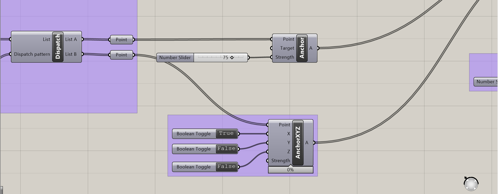
1. An “Anchor” component was used to anchor inside points to the base.
2. An “Anchor XYZ” component was used to avoid stretching edge lengths and give some structure to the arches. However, in the end, I decided not to use the anchor for the Y and Z axis for the functionality and aesthetics of the design.

Step 4

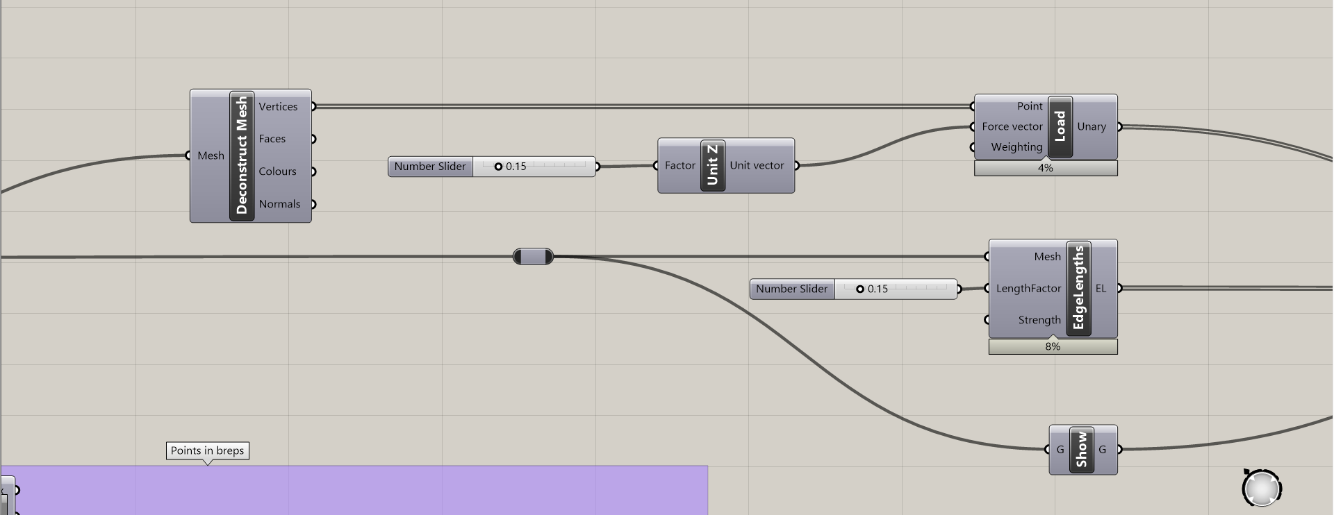
1. Using the Kangaroo plugin, the initial mesh was plugged into “Edge Lengths”, and the factor was set to 0.15.
2. To place load onto the mesh vertices, “Deconstruct Mesh” was used to define the vertices and then plugged into the “Load” component.
3. To simulate the spring factor, the “Unit Z” component was plugged into “Load” and given a suitable factor of 0.15.
4. Finally, the “Show” component was used to view it in the final simulation.

Step 5

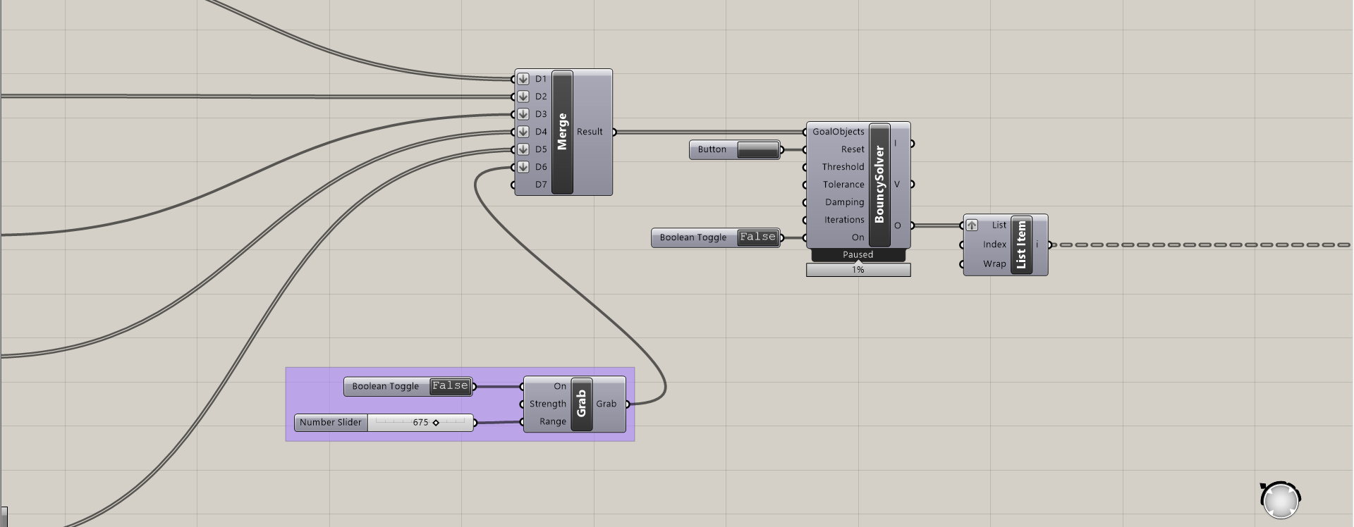
1. The components’ output was then merged using the “Merge” component and plugged into “Bouncy Solver” to start the simulation, with the help of a reset button and boolean toggle.
2. Next, the “List Item” component subdivided the mesh surface into grids with the help of the “Mesh to Ploysurface” component from the Lunchbox plugin.
3. As a fun part, I like to use the “Grab” component to play around with the shell.

Step 6

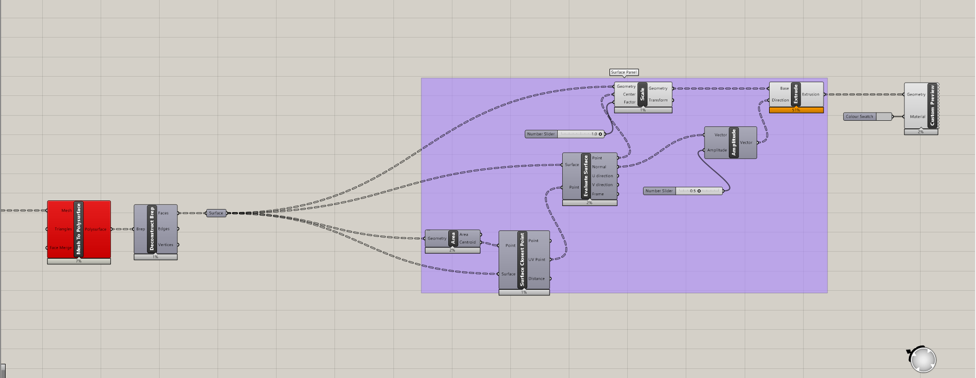
1. After subdividing the mesh surface, it was plugged into “Deconstruct Brep” to break down into faces and vertices, and the resultant surface could be used to work out the thickness of the concrete shell.
2. The surface is plugged into “Area” to get a centre point for each surface on the grid. Since this is not an accurate centre point, “Surface Closest Point” was used to get the accurate points.
3.  Next, I used “Evaluate Surface” and “Scale” to further detail the modular units utilising a number slider.
4. To extrude the shell and give it a thickness, the “Extrude” component was used along with “Amplitude” to manage the vector value.
5. At last, a simple “Custom Preview” was used to set the colour and graphics of the final result, as shown below.

I am attaching the grasshopper and rhino files to understand this exercise better.