1 INTRO
We have always designed space by intuition, rarely quantifying the rules that govern it. What if instead, space designed itself — guided not by a hand, but by the encoded logic of architectural knowledge translated into force?
This project explores the automated generation of apartment floor plans through physics-based simulation rather than rule-based. A boundary curve and a set of room requirements are the only inputs — the system handles the rest. The result is a fully parametric configurator running natively in Grasshopper/Rhino.
2 INSPIRATION + RESEARCH
The work draws on space syntax theory and residential planning norms to ground the generation process in architectural principles rather than pure geometry. Research into Polish and Czech building standards informed area targets, room adjacency requirements, and circulation logic. Existing configurator tools were surveyed to identify the gap between freeform optimization and norm-compliant layout generation. Main inspiration cames from emarching softwares for appartment designs such as : https://www.finch3d.com
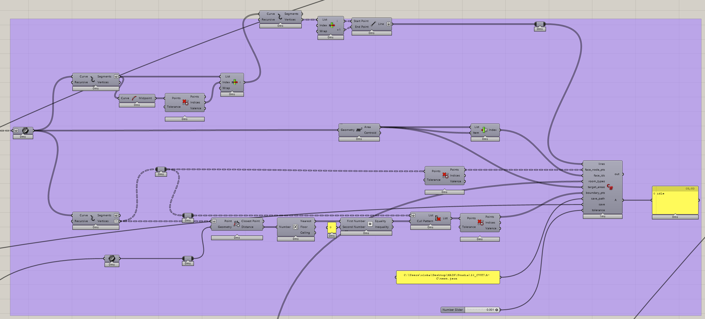
3.0 TECHNOLOGY
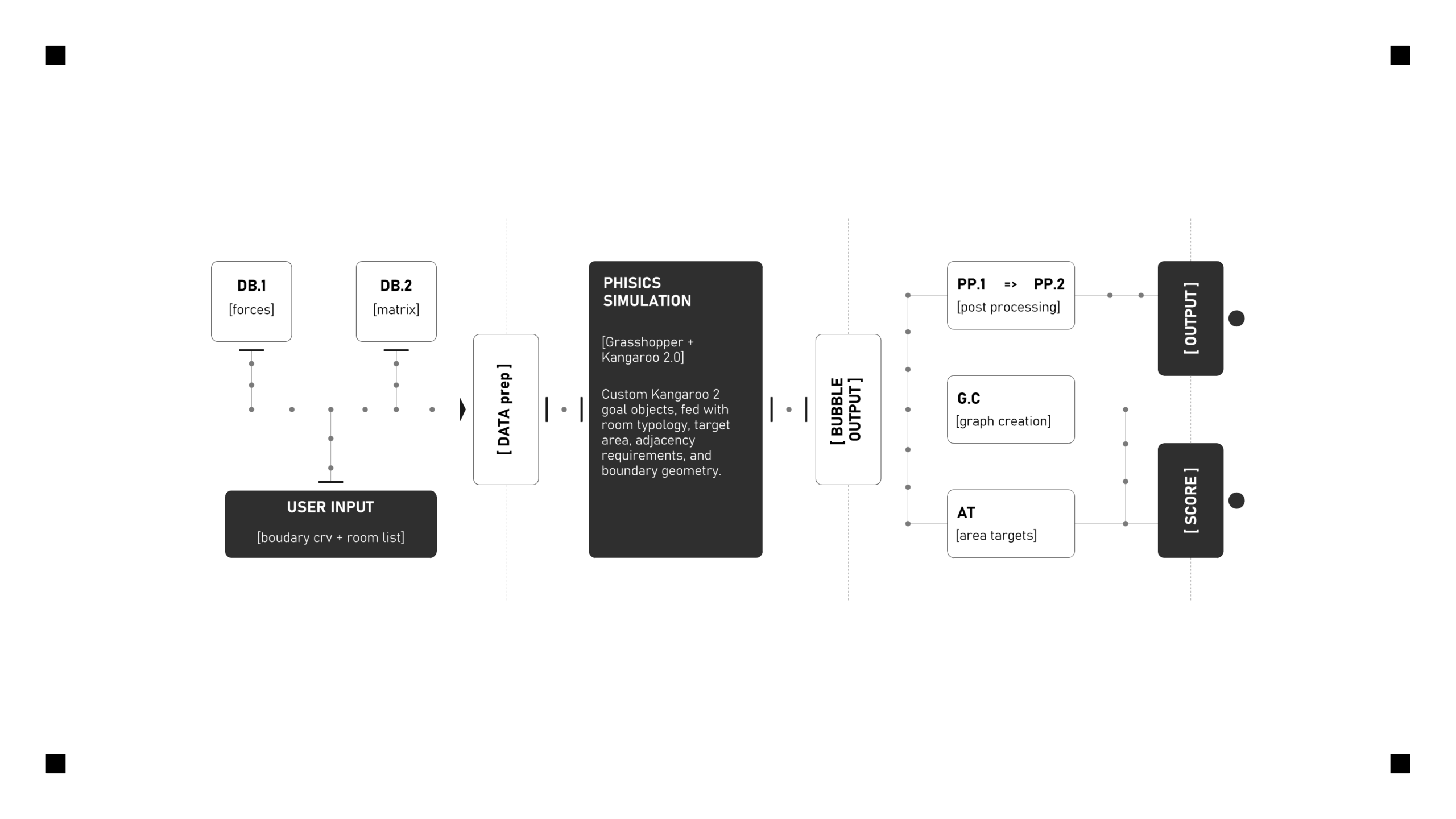
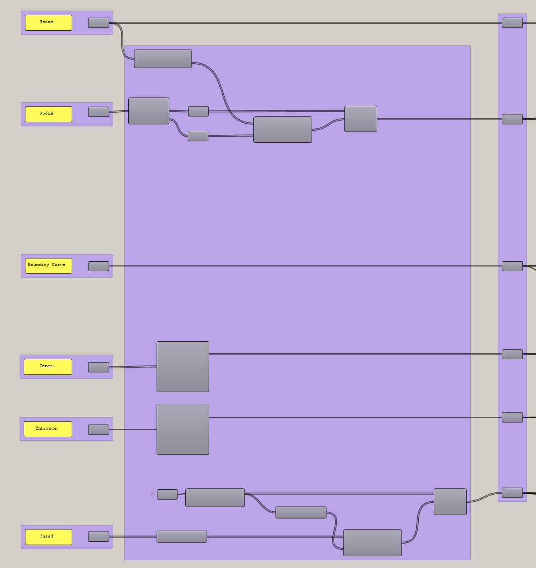
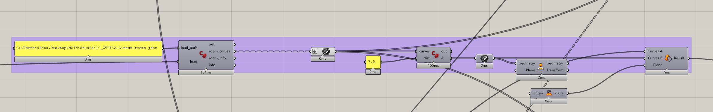
The pipeline is built entirely in Grasshopper using C# Script and Python components, with Kangaroo 2 as the physics solver. No external AI or ML libraries are involved — all intelligence is encoded as explicit goals, constraints, and scoring logic. JSON serialization handles data transfer between simulation stages without relying on any third-party parsing libraries.
3.1. PARAMS INTRODUCTION
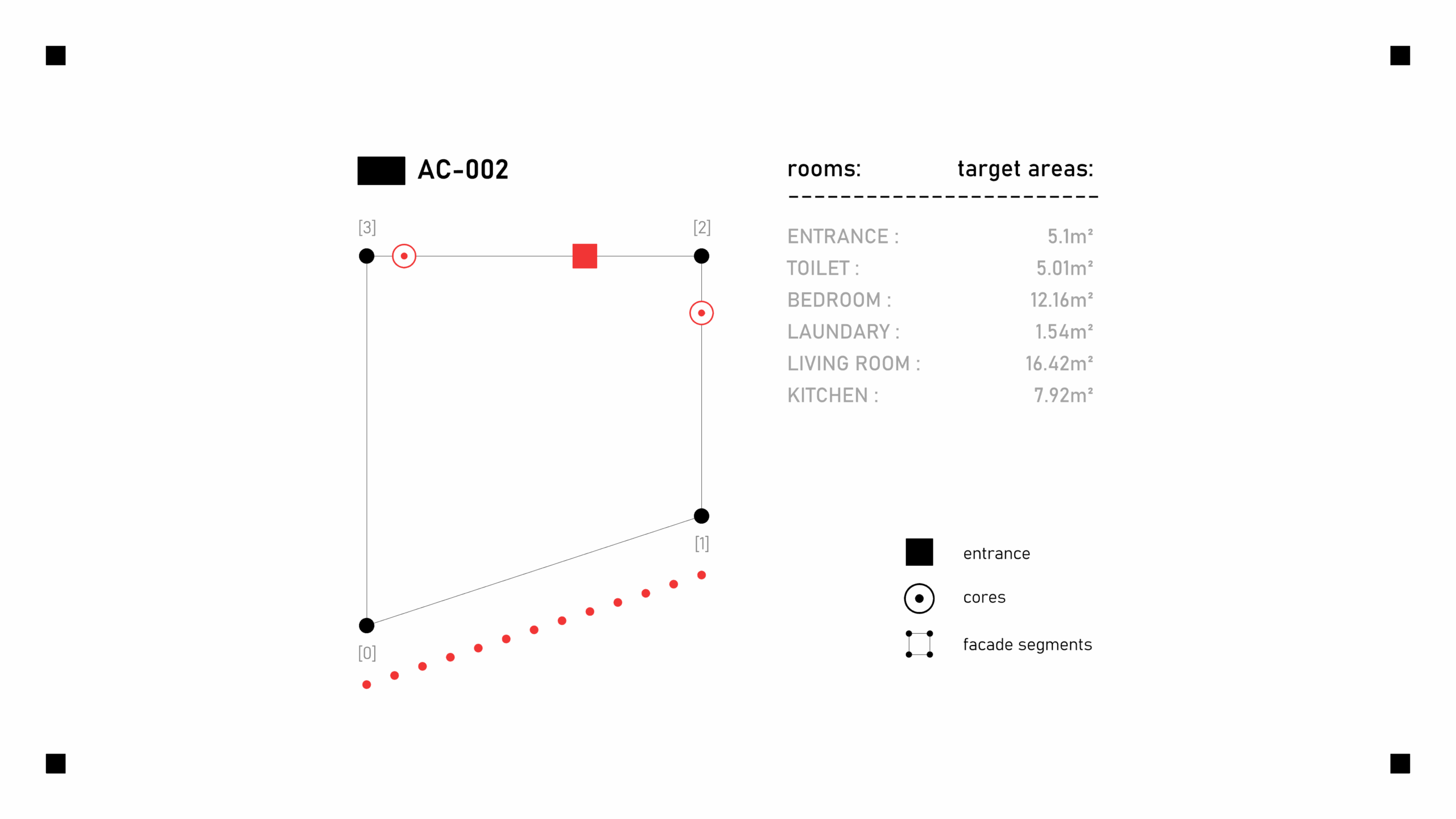
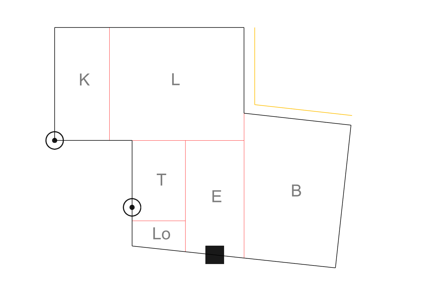
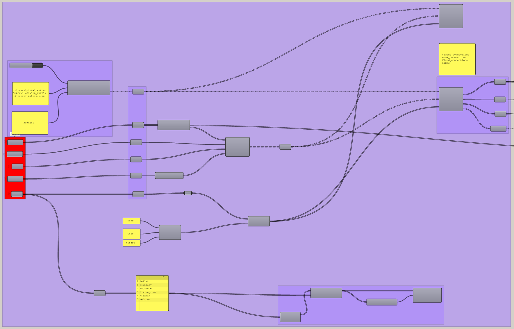
Users define an apartment boundary curve and a list of rooms with target areas and adjacency preferences. Two input modes are supported: manual parameter entry for custom configurations(fig.1), and a reference mode that loads real apartment layouts for benchmarking(fig.2). This dual approach allows both free exploration and validation against built examples.
3.2 PRESET DATABASES
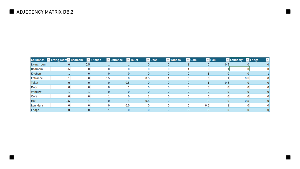
A database of room type presets encodes typical area ranges and adjacency weights drawn from residential building norms. These presets are loaded as structured data and feed directly into the simulation setup, reducing manual configuration. The database can be extended to cover different apartment typologies or national standards. (fig.1)
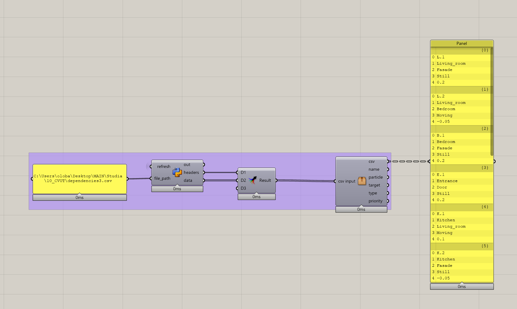
3.3 SORTING AND DATA PREPARATION
Room requirements are sorted and preprocessed before simulation to establish initial particle positions and goal hierarchies. Boundary sampling and adjacency matrix construction happen at this stage, outputting structured DataTrees consumed downstream. This preparation step is critical — malformed topology here propagates as unfixable artifacts in post-processing.
For Kangaroo set up the workflow divides goals basing on 5 different types:
- static goals (collisions, rigid body, )
- 2D inflation
- Kinetic goals 1 (attraction/repulsion to moving objects)
- Kinetic goals 2 (attraction/repulsion to static point elements)
- Kinetic goals 3 (attraction/repulsion to static line elements)
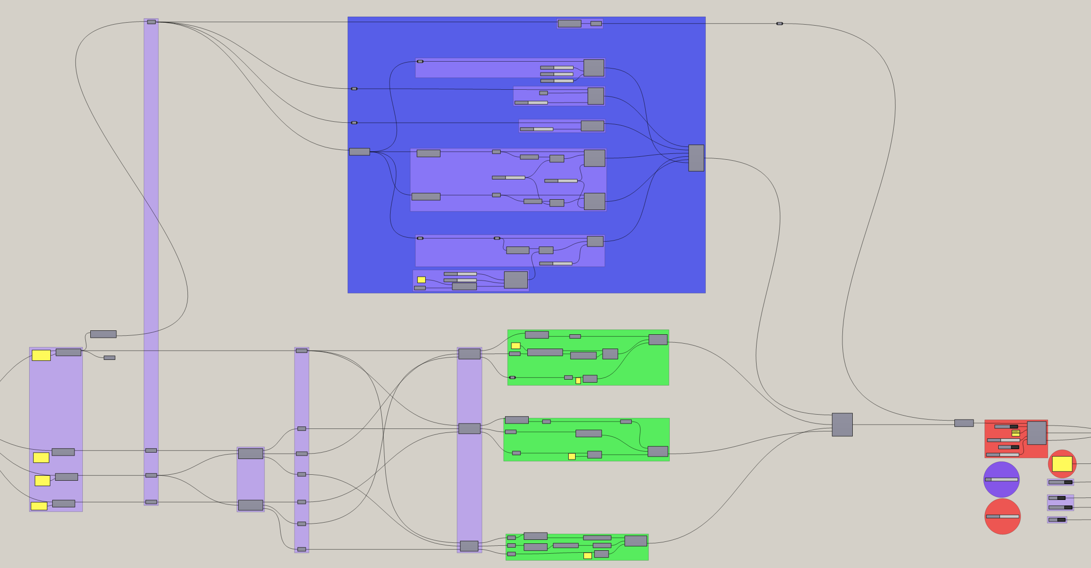
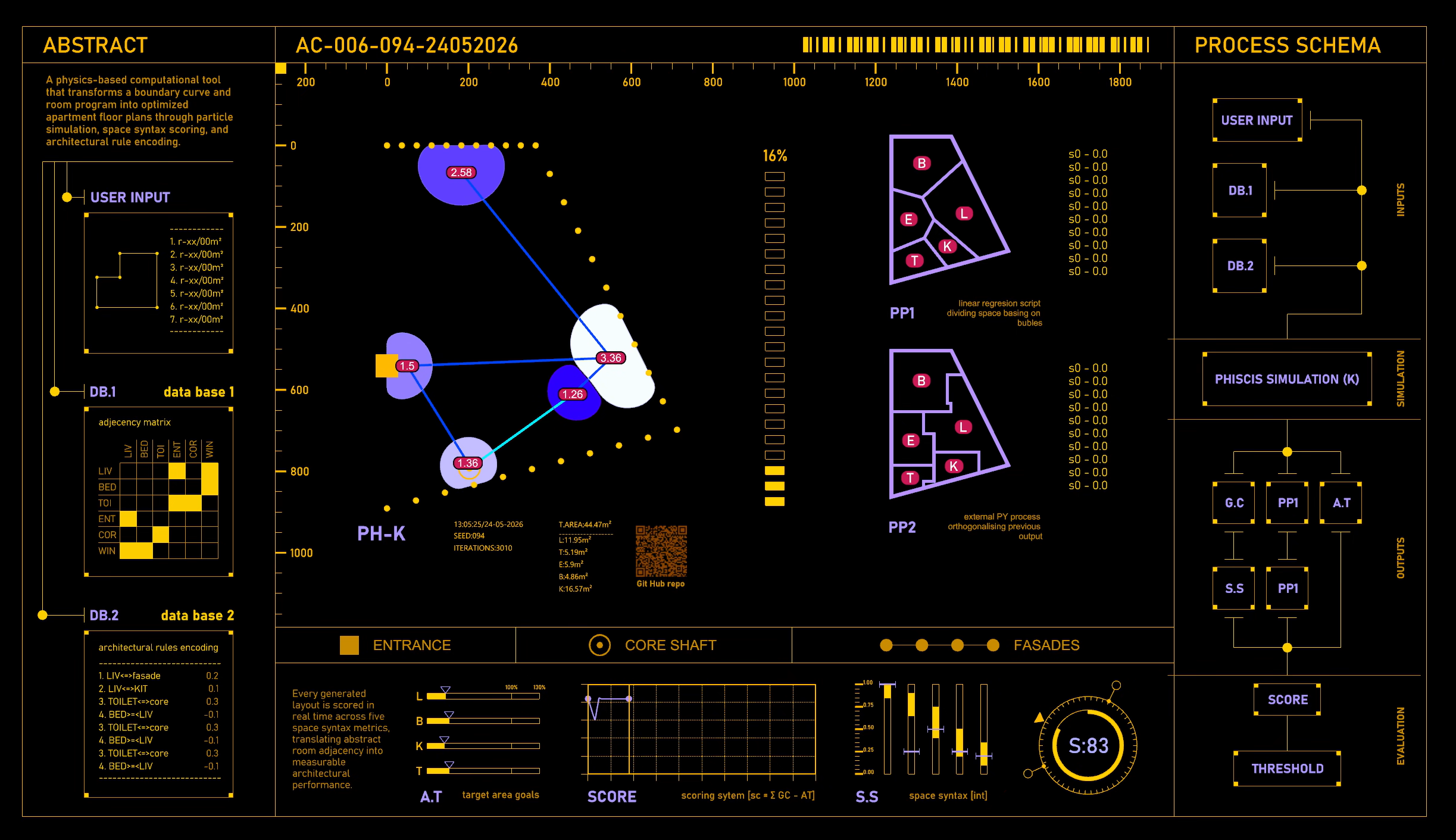
3.4 SIMULATION
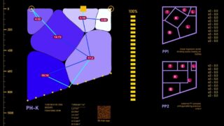
Room centroids are modeled as particles in a Kangaroo 2 solver, driven by attraction/repulsion goals that enforce adjacency preferences and area targets. The solver runs iteratively, converging toward a bubble diagram where spatial relationships satisfy the encoded constraints. Goal objects are cached and updated each tick rather than rebuilt, ensuring forces always calculate from current positions.
4.0 GRAPH CONSTRUCTION
Once the simulation converges, the bubble diagram is parsed into a planar graph by detecting adjacencies between settled particles. Node positions and edge topology are extracted and exported as JSON for downstream processing. This graph is the backbone for both orthogonalization and space syntax scoring.
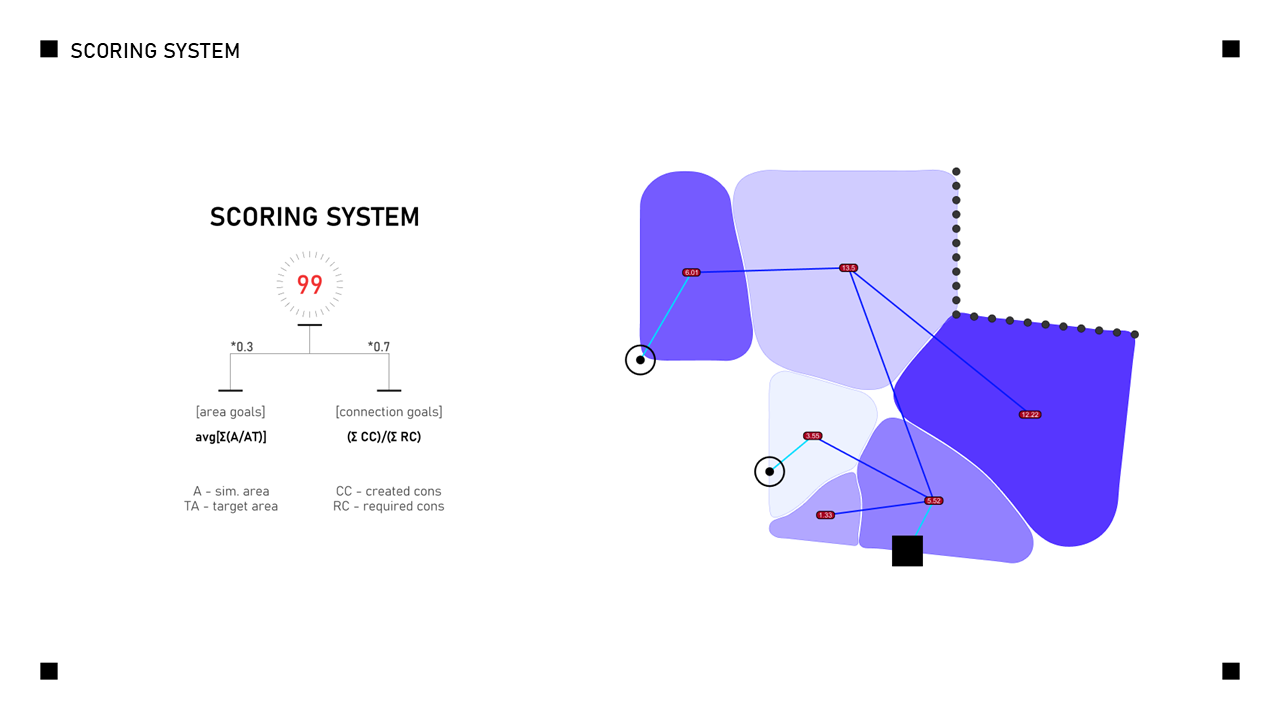
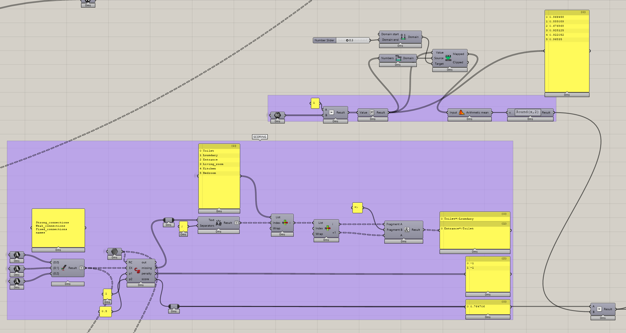
5.0 SCORING SYSTEM
Each generated layout is evaluated against a composite score combining space syntax integration values, adjacency satisfaction, and area deviation from targets. The scoring runs automatically across the population of generated variants, enabling objective comparison. Results are ranked and visualized in-viewport using custom 2D text rendering components.
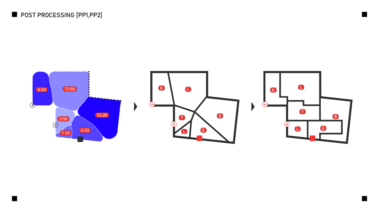
6.0 POST PROCESSING
The bubble graph is converted into an architectural floor plan firstly through linear regression script that outputs “voronoi like” space division and then a Python-based orthogonalization pass using Shapely. A cut grid derived from all node coordinates seeds room polygons, which are then grown to target areas with sliver merging and compactness scoring. Wall geometry is generated from boundary offsets and junction snapping, with dead-end connections resolved back to the apartment boundary.
//there are some ambiguities concerning few thresholds while cleaning the data during PP.1
//thats the only instance where script requires user interference
7.0 FINAL UI
The complete pipeline is exposed through a single Grasshopper interface that consolidates parameter input, simulation control, scoring display, and geometry output. Visual feedback is rendered directly in Rhino viewports. The interface is designed to remain legible during live simulation without requiring Rhino restarts between iterations. This way the script is quicker and has the ability to record all of the results well sorted in .json file which u can see here : https://github.com/barnasiunnio/AC-Physic-Simulation
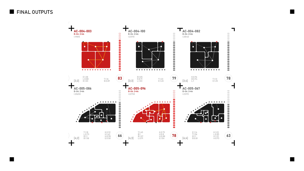
8.0 RESULTS ANALYSIS
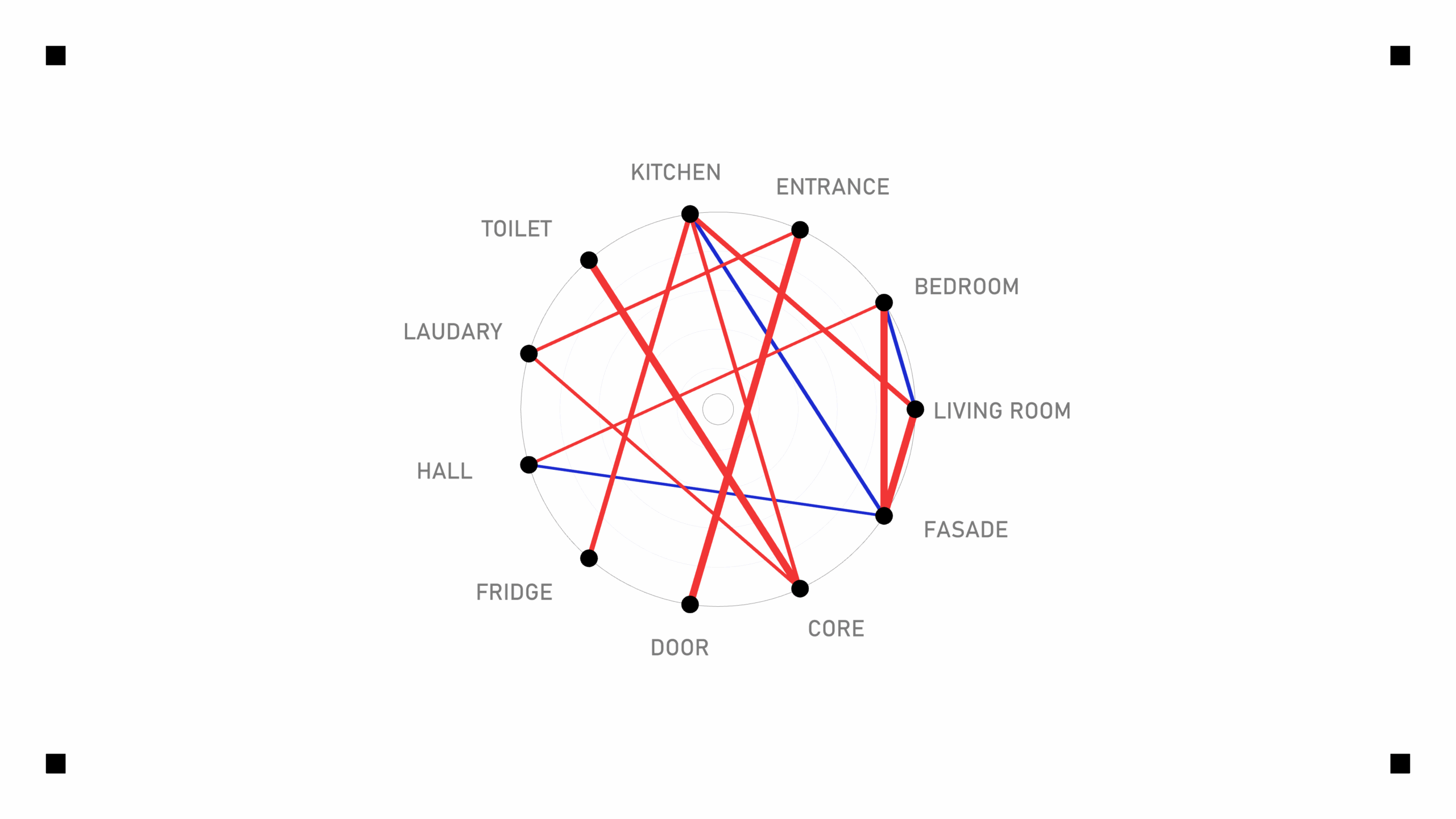
Generated floor plans are evaluated side-by-side against reference apartments from the Florence 21 housing dataset. Adjacency matrices, area tables, and space syntax graphs are output as structured data for further analysis. The comparison reveals how closely physics-driven generation can match norm-compliant hand-designed layouts hence how well the script performs (providing the floorplans from Florence 21 are well designed :))
9.0 EXTRAS
One of the most demanding aspects of the project was managing a multi-goal Kangaroo 2 simulation where attraction, repulsion, boundary containment, and area-scaling forces had to coexist without destabilizing the solver. Goal weight tuning proved highly sensitive — small changes in one goal would cascade into oscillation or topology collapse elsewhere, and the Grasshopper C# environment added constraints around goal caching, particle registration, and per-tick update logic that made iteration slow. For future development, migrating the entire simulation stage to Python — likely via a dedicated physics library — would significantly improve debuggability, scriptability, and the ability to run headless batch optimizations outside of the Grasshopper canvas.